Course2-week1-setting up your ML application

setting up your ML application

1 - train/dev/test set

This week we’ll learn the partical aspects of how to make your neural network work well, ranging from things like hyperparameters tuning to how to set up your data, to how to make your optimization algorithm runs quickly.

Making a good choice in how you set up your training, development, test set can make a huge different in helping you quickly find a good high performance neural network. When you starting off a new application it’s almost impossoble to correct guess the right value for all of the parameters, such like #layer, #units, learning rate, activation function on your first attemp. So in partice applied machine learning is a highly iterative process.

Traditionally you might take all the data you have and carve off some portion of it to be training set, some portion of it be your hold-out cross validation set, also called the development set, and carve off final portion of it to be your test set. And so the workflow is that you keep on training algorithms on your training set, and use dev set to see which of many different models performs best on your dev set, and having done this long enough, when you have a final model you want to evaluate, you can take the best model you find and evaluate it on your test set in order to get an unbiased estimate of how well your algorithm is doing.

In the previous era of machine learning, it was common partice to take all your data to split it according to 70/30 train/test split if you don’t have explicit dev set or maybe 60/20/20%.But in the modern big data era, the trend is that your dev set and test set have been becoming a much small percentage of the total. Because the goal of the dev set is that you are going to test different algorithms on it and see which algorithms works better. And the main goal of your test set is to give your final classifier a pretty confident estimate of how well it’s work. So if you have a relative small dataset, the traditional ratios might be okay, But if you have a much big dataset, it also fine to set your dev and test set to be nuch small, for example 98/1/1 or 99/0.5/0.5%.

One other trend we are seening in the era of modern deep learning is that more and more prople train on mismatched train and test distributions, Let’s say you are building an app that lets users uploads a lot of pictures, and your goals is to find picture of cats in order to show your users, maybe your users all cat lovers, maybe be your training set come from cat picture downloads off the Internet, but your dev and test set might comprise the cat pictures from users’ upload useing our app. So these two distributions of data may be different. The rule of thumb I’s encourage you to follow in this case is to make sure that dev and test set come from the same distribution. Because you will be use the dev set to evaluate a lot of different models and try really hard to improve performance on the dev set. It’s nice if your dev set comes from the same distribution as your test set. Finally, it’s maybe okay to not have a test set, remember the goal of test test is to give you a unbiaed estimate of the performance of your final model that your select through dev set. If you don’t need unbiased estimate, it’s okay to not have test set. So what you do, If you have only a dev set but not a test set, is that you training on the training set and then try different model architecture evaluate them on the dev set and iterate try to get a good model, because you fit data in your dev set, this no longer gives you an unbiased estimate of performance. In this case, people usually call the dev set the test set, but what they end up actually doing is using the testing set as dev set.

So have set the train/dev/test set allow you to more efficiently measure the bias and the variance of your algotithm, so you can more efficiently select the ways to improve your algorithm.

2 - bias & variance

In deep learning error, there’s less of a trade-off, We still solve the bias, and still solve the variance, but just talk less about the bias-variance trade-off.

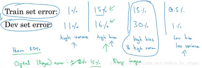
The two key numbers to look at to understand bias and variance wil be the train set error and the test set error.

• high variance: you might have overfit the training set and that somehow you are not generalizing well on the dev set.
• high bias:(assuming that humans achieve roughly 0% error)the algorithm not even doing well on the training set, but in constast, this actually generalizing at a reasonable level to the dev set.
• high bias and high variance:it’s not doing well on the training set, so high biase, and the perfomance on the dev set much worse than the performance on the train set, so high variance.
• low bias and low variance:

This analysis is on the assumption that human level performance that get nearly 0% error. The optimal error, sometimes called Bayes error.

By looking at your training set error, you can get a sense of how well you are fitting, at least the training set data, and so that tells you if you have a bias problem. And then looking at how much higher your error goes when you go from the train set to the dev set, that should give you a sense how bad is the variance problem. All this is under the assumption that the Bayes error is quite samll and your train and dev set are come from the same distribution.

What’s high bias and high variance look like?

Where it has high bias, because it was mostly linear, but you maybe need a curve function or a quadratic function, and it has high variance, because it has too much flexibility to fit the mislabel example.

Now we have seen how by looking at the algorithm error on the training set and dev set to diagnose whether it has problems of high bias or high variance or maybe both, or maybe neither. And depending on whether your algorithm suffer from bias and variance, it turn out the different things you could try.

3 - basic recipe for machine learning

Depending on whether you have high bias or high variance, the second things you would be try could be quite different.

• high bias:
  
  • bigger network
  • train longer time
  • (find some appropriate neural network architecture)
• high variance:
  
  • get more data
  • regularization
  • (find some appropriate neural network architecture)

In the earlier era of machine learning,there used to be a lot of discussion on what is called the bias and variance tradeoff, and the reason for that is for a lot of things you could try you could increase bias and reduce variance or increase variance and reduce bias, we didn’t have the tools that just reduce bias or just reduce variance without hurt the other one. But in the modern deep learning era, so long as you can keep training a bigger network and so long as you can keep getting more data, getting a bigger network almost always just reduce your bias without hurt your variance, so long as you regularize appropriately. And getting more data pretty always reduce your variance and doesn’t hurt your bias much. So last you have a well regularized network and training a bigger network almost never hurts.

4 - regularization

If you suspect your neural network is over fitting your data, that is have a high variance problem, one of the first thing you should try is regularization. Let’s see how regularization work.

for logistic regression:

J(w,b)=1m∑i=1mL(y^(i),y(i))+λ2m∥w∥22 J ( w , b ) = 1 m ∑ i = 1 m L ( y ^ ( i ) , y ( i ) ) + λ 2 m ‖ w ‖ 2 2

where:

∥w∥22=wTw=∑j=1nxw2j ‖ w ‖ 2 2 = w T w = ∑ j = 1 n x w j 2

∥w∥22 ‖ w ‖ 2 2 called the L2 regularization with the parameters vector w w .

L2 L 2 regularization is the most common type of regularization.

L1 regularization:

λ2m∥w∥1=λ2m∑j=1nx|wj| λ 2 m ‖ w ‖ 1 = λ 2 m ∑ j = 1 n x | w j |

If we use L1 regularization, w w will end up being sparse. But when people training network, L2 regularization is just used much much more often. λ λ is another hyperparameter you have to tune to trading off between doing well in your training set versus also setting the regularization items to be small.

for neural network:

J(W[1],b[1],⋯,W[L],b[L])=1m∑i=1mL(y^(i),y(i))+λ2m∑l=1L∥W[l]∥2F J ( W [ 1 ] , b [ 1 ] , ⋯ , W [ L ] , b [ L ] ) = 1 m ∑ i = 1 m L ( y ^ ( i ) , y ( i ) ) + λ 2 m ∑ l = 1 L ‖ W [ l ] ‖ F 2

where:

∥W[l]∥2F=∑i=1n[l]∑j=1n[l−1](w[l]ij)2 ‖ W [ l ] ‖ F 2 = ∑ i = 1 n [ l ] ∑ j = 1 n [ l − 1 ] ( w i j [ l ] ) 2

This matrix norm is called Frobenius norm of matrix

So how the implement gradient descent with this?

W[l]=W[l]−αdW[l](1) (1) W [ l ] = W [ l ] − α d W [ l ]

where :

dW[l]=(from backpropagation) d W [ l ] = ( f r o m   b a c k p r o p a g a t i o n )

this is before we added this regularization term to the objective, after added the term.

dW[l]=(from backpropagation)+λmW[l] d W [ l ] = ( f r o m   b a c k p r o p a g a t i o n ) + λ m W [ l ]

now the equation (1) becomes to:

W[l]=W[l]−α((from backpropagation)+λmW[l])=W[l]−α(from backpropagation)−αλmW[l]=W[l](1−αλm)−αdW[l] W [ l ] = W [ l ] − α ( ( f r o m   b a c k p r o p a g a t i o n ) + λ m W [ l ] ) = W [ l ] − α ( f r o m   b a c k p r o p a g a t i o n ) − α λ m W [ l ] = W [ l ] ( 1 − α λ m ) − α d W [ l ]

So this is why L2 regularization is also called weight decay, because now we are multipling W W by (1−αλm) ( 1 − α λ m ) which is a little bit less than 1.

5 - why regularization reduces overfitting?

Why does regularization help with overfitting, why does it help reducing variance problem?

J(W[1],b[1],⋯,W[L],b[L])=1m∑i=1mL(y^(i),y(i))+λ2m∑l=1L∥W[l]∥2F J ( W [ 1 ] , b [ 1 ] , ⋯ , W [ L ] , b [ L ] ) = 1 m ∑ i = 1 m L ( y ^ ( i ) , y ( i ) ) + λ 2 m ∑ l = 1 L ‖ W [ l ] ‖ F 2

What we did for regalarization was add extra term that penalizes the weight matrix from being too large. So why is it the Frobenius norm of parameters might cause less overfitting?

one piece of the intuition is if you crank regularization λ λ to be really large, this will incentivized to set the weight matrices W W to be close to zero. This’s basically zeroing out a lot of the impect of these hidden units. This much simplier neural network to becomes a much smaller neural network. That will take you from the overfitting case to the high bias case. And hopefully these will be an intermediate value of λ λ that result in a result closer to just fitting case in the middle.

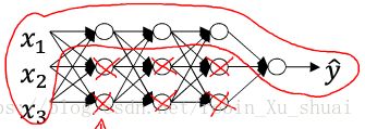
The intuition of completely zeroing out a bunch of hidden units isn’t quite really. It turn out that what actually happens is they’ll still use all the hidden units, but each of them would just have a much smaller effect, you do end up with a simplier network, as if you have a smaller network there’s less to overfitting.

If every layer is linear, then your whole network is just a linear network, and so even a very deep network with a linear activation function at the end they are only be able to compute a linear function. So it's not able to fit the very complicated non-linear decision boundaries.

if the regularization parameter λ λ become very large, the parameter W W will be very small, Z Z will be small, it takes on a small range of values, so the activation function if is tanh will be relatively linear. And the whole network will be computing something not too far from a big linear function rather than a very compelx highly non-linear function.

6 - dropout regularization

Another very powerful regularization techniques is called “dropout”.

With dropout, what we are going to do is go through each of the layers of the network, and set some probability of eliminating a node in neural network. For each node, we are going to toss a coin, and have some chance of keeping each node and some chance of removing each node, so after the coin toss, maybe we will decide to eliminate some nodes. And then what you do is actually remove all the ingoing outgoing things from that nodes as well. So we end up with a much smaller, really much diminished network. And then do back propagation, training this one example on this much diminished network. And on different examples, we would toss a set of coins again and keep a different set of nodes and then dropout different set of nodes, So for each training example, we would train it using one of neural reduced networks.

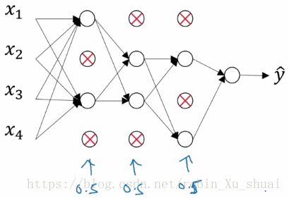
inverted dropout:

Now we will illustratin how to implement dropout in a single layer.

set a vector d3 d 3 going to be the dropout vector for the layer 3,

d3 = np.random.rand(a3.shape[0], a3.shape[1]) < keep_prob
a3 = np.multiply(a3, d3) # element wise multiplication a3 *= d3
a3 /= keep_prob

let me explain what this final step is doing. **Let’s say you have 50 units in layer 3, so the a3 is 50 by m dimensional. So if we have a 20% chance of eliminating them, this means that on average, we end up with 10 units zeroed out. Due to Z[4]=W[4]a[3]+b[4] Z [ 4 ] = W [ 4 ] a [ 3 ] + b [ 4 ] , a[3] a [ 3 ] will be reduced by 20%, So in order to not reduce the expected value of Z[4] Z [ 4 ] , what you need to do is to implement the final step. a3 /= keep_prob is what’s called the **inverted dropout technique.

So what we do is use the d d vector, and we will notice that for different training examples, we zero out different hidden units. And in fact, if you make multiple passes through the same training set, will randomly zero out different hidden units.

Having trained the algorithm, here’s what we would do at test time is not to use dropout at test time.

7 - understanding dropout

We have know that the dropout randomly knocks out units in your neural network, so it’s as if on every iteration, you are working with a smaller neural network, and so using a smaller neural network seems like it should have a regularizing effect.

Why does dropout work?

Another Intuition: one units can't rely on any one input feature of it, so have to spread out weights. By spreading all the weights, this will tend to have an effect of shrinking weight, so that dropout has show the similiar effect to L2 regularization. Only the L2 regularization applied to different weights can be a little bit different and even more adaptive to the scale of different inputs.

These could be different keep_prob for different layer, Notice that the keep_prob = 1.0 means that you are keeping every unit and so you are really not using dropout for that layer. Bor for layer where you are more worried about overfitting, the layers with a lot of parameters, you can setkeep_prob smaller to apply a more powerful form of dropout.

Dropout is a regularization technique it helps prevent overfitting. So unless algorithm is overfitting, we wouldn’t actually bother to use dropout. So it’s used less often than other application areas. There’s just for computer version, you usually don’t have enough data, so you’re almost always overfitting.

8 - other regularization methods

data augmentation can be used as a regularization technique.This can be an inexpensive way to give your algorithms more data.

early stopping :
when you haven’t run many iterations for your network yet, the parameters will be close to 0. And then as your iterate, the w w get bigger and bigger. So what early stopping does is by stopping halfway we have mid-size ∥w∥F ‖ w ‖ F .

Early stopping does have one downside. The machine learning process are comprising serveral different steps.

• you want a algorithm to optimize the cost function J J , we have various tools to do that, such as gradient descent, momentum and RMSprop and Adam and so on.
• after optimizing the cost J J , we also wanted to not overfitting, we have also some tools to do that such as regularizations, getting more data and so on.

The main downsides of early stopping is that this cope with these two tasks, so you no longer can work on these two tasks problem independently, because by stopping gradient descent early, you are sort of breaking whatever you are doing to optimize cost J J , because you are not doing a good job reducing the cost function. And then you also simultaneously trying to not overfitting. Instead of using different tools to solve the two tasks. In contrast, other technique of regularization, L2 regularization, allow you to train your neural network as long as possible.

9 - normalizing input

when you train your neural network, one of the techniques that will speed up your training is if normalize your input.

Normalizing your input corresponds to two step:

• subtract out mean
  
  • μ=1m∑mi=1x(i) μ = 1 m ∑ i = 1 m x ( i ) where σ2 σ 2 is a vector with the means of each of the feature
    • x−=μ x − = μ for each training example
    • normalize the variance
      
      • σ2=1m∑mi=1x(i)∗∗2 σ 2 = 1 m ∑ i = 1 m x ( i ) ∗ ∗ 2 where σ2 σ 2 is a vector with the variances of each of the feature
      • x/=σ x / = σ

    • 
      

      And one tip, if you use this to scale your training data, then use the same μ μ and σ σ to normalize your test set, rather than estimating μ μ and σ σ separately on your training set and testing set.

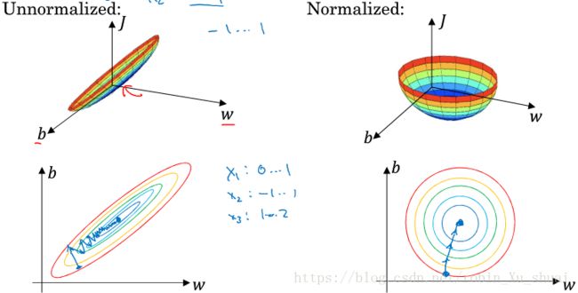
      So why do we want to normalize the input feature?

      If your features are on very different scale, the feature x1 x 1 ranges from 0 to 1,and feature x2 x 2 ranges from 1 to 1000, it’s turns out the range of parameter w1 w 1 and w2 w 2 will end up taking on very different values. The rough ituition that your cost function will be more round and easier to optimize when your feature are all on the same scales, and will usually help your learning algorithm run faster.

      
      

      10 - vanishing/exploding gradient

      When you training a very deep network, your slopes can sometimes get either very big or very small, both these make training difficult.
      

      
      

      For the sake of simplicity, let’s say we will using an activation function g(z)=z g ( z ) = z and ignore b b . In that case we will show that

      y^=W[L]W[L−1]⋯W[3]W[2]W[1]X y ^ = W [ L ] W [ L − 1 ] ⋯ W [ 3 ] W [ 2 ] W [ 1 ] X

      let’s say that except the last one, the rest of these weight matrices is:

      W[l]=[1.5001.5](5) (5) W [ l ] = [ 1.5 0 0 1.5 ]

      That will have:

      y^=W[L][1.5001.5][L−1]X=W[L]1.5[L−1]X(6) (6) y ^ = W [ L ] [ 1.5 0 0 1.5 ] [ L − 1 ] X = W [ L ] 1.5 [ L − 1 ] X

      conversely, if we replace 1.5 with 0.5

      W[l]=[1.5001.5](7) (7) W [ l ] = [ 1.5 0 0 1.5 ]
      y^=W[L][0.5000.5][L−1]X=W[L]0.5[L−1]X(8) (8) y ^ = W [ L ] [ 0.5 0 0 0.5 ] [ L − 1 ] X = W [ L ] 0.5 [ L − 1 ] X

      So if the weights W[l]>I W [ l ] > I , with a deep network, the activation can be explode, if W[l]<1 W [ l ] < 1 , the activation will decrease exponentially. And the same augment can be used to show that the gradient will also increase exponentially or decrease exponentially as a function of the number of layers.

      11 - weight initialization for deep networks

      Now we saw how very deep neural networks can have the problems of vanishing and exploding gradient, it turns out that a partial solutions to this is better or more careful choice of the random initialization for your neural network.

      z=w1x1+w2x2+⋯+wnxn z = w 1 x 1 + w 2 x 2 + ⋯ + w n x n

      So in order to make z z not blow up and not become too small, we notice that the large n is, the smaller we want wi w i to be. One reasonable thing to do would be to set the variance of wi w i to be equal to 1n 1 n . Var(wi)=1n V a r ( w i ) = 1 n

      In partice:

      W[l]=np.random.randn(W[l].shape)∗np.sqrt(1n[l−1]) W [ l ] = n p . r a n d o m . r a n d n ( W [ l ] . s h a p e ) ∗ n p . s q r t ( 1 n [ l − 1 ] )

      if the activation function you used is Relu, rather than set the Var(wi) V a r ( w i ) to be 1n 1 n , the 2n 2 n maybe a better choice.

      W[l]=np.random.randn(W[l].shape)∗np.sqrt(2n[l−1]) W [ l ] = n p . r a n d o m . r a n d n ( W [ l ] . s h a p e ) ∗ n p . s q r t ( 2 n [ l − 1 ] )

      If the activation value are roughly mean 0 and variance 1, then this would cause z z to also take on a similiar scale. And this doesn’t solve, but helps reduce the vanishing and exploding gradient problems, because it’s try to set the weights matrice w w not too much big than 1, and not too much less than 1, so it doesn’t exploding and vanishing too qucikly.

      if you are using a tanh function:
      

      1n[l−1]−−−−−√ 1 n [ l − 1 ]
      
      this called xavier initialization, or:
      
      2(n[l−1]+n[l])−−−−−−−−−−−√ 2 ( n [ l − 1 ] + n [ l ] )

      12 - numerical approximation of gradient

      Gradient check can really help you make sure that your implementation of back propagation is correct. How to numerically approximate computation of gradients.

      
      
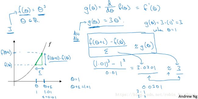      f(θ)=θ3 f ( θ ) = θ 3
      
      
      g(θ)=ddθf(θ)=f′(θ)=3θ2 g ( θ ) = d d θ f ( θ ) = f ′ ( θ ) = 3 θ 2
      
      
      g(1)=3 g ( 1 ) = 3
      f(θ+ϵ)−f(θ)θ≈g(θ) f ( θ + ϵ ) − f ( θ ) θ ≈ g ( θ )
      
      
      1.013−130.01=3.0301≈3 1.01 3 − 1 3 0.01 = 3.0301 ≈ 3

      approx error = 0.0301

      
      

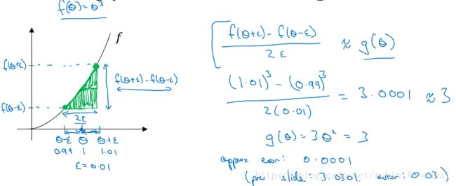
      Rather than a one side difference, we are taking a two side difference.

      f(θ+ϵ)−f(θ−ϵ)2ϵ≈g(θ) f ( θ + ϵ ) − f ( θ − ϵ ) 2 ϵ ≈ g ( θ )
      
      
      1.013−0.9930.02=3.0001≈3 1.01 3 − 0.99 3 0.02 = 3.0001 ≈ 3

      approx error = 0.0001

      ---

      f′(θ)=limitϵ−>0f(θ+ϵ)−f(θ−ϵ)2∗θ error:O(ϵ2) f ′ ( θ ) = l i m i t ϵ − > 0 f ( θ + ϵ ) − f ( θ − ϵ ) 2 ∗ θ   e r r o r : O ( ϵ 2 )
      
      
      f′(θ)=limitϵ−>0f(θ+ϵ)−f(θ)θ error:O(ϵ) f ′ ( θ ) = l i m i t ϵ − > 0 f ( θ + ϵ ) − f ( θ ) θ   e r r o r : O ( ϵ )

      We need to take away is that two-side different formula is much more accurate. So that’s what we are going to use when we do gradient checking.

      13 - gradient checking

      To implementation gradient checking, the first thing we need to do is take all parameters W[1],W[1],⋯,W[L],b[L] W [ 1 ] , W [ 1 ] , ⋯ , W [ L ] , b [ L ] and reshape them into a giant vector θ θ . Next with W W and b b ordered the same way, take dW[1],db[1],dW[2],⋯,dW[L],db[L] d W [ 1 ] , d b [ 1 ] , d W [ 2 ] , ⋯ , d W [ L ] , d b [ L ] and reshape into a giant vector dθ d θ .

      implement grad checking:

      for all the compontent i i in θ θ

      dθapprox[i]=J(θ1,θ2,⋯,θi+ϵ,⋯)−J(θ1,θ2,⋯,θi−ϵ,⋯)2ϵ≈dθ[i] d θ a p p r o x [ i ] = J ( θ 1 , θ 2 , ⋯ , θ i + ϵ , ⋯ ) − J ( θ 1 , θ 2 , ⋯ , θ i − ϵ , ⋯ ) 2 ϵ ≈ d θ [ i ]

      at the end, you end up two vector, dθapprox d θ a p p r o x and dθ d θ

      What we going to do is check if these vector are approximately equal to each other.

      ∥dθapprox−dθ∥2∥dθapprox∥2+∥dθ∥2=r ‖ d θ a p p r o x − d θ ‖ 2 ‖ d θ a p p r o x ‖ 2 + ‖ d θ ‖ 2 = r

      where ϵ=10−7 ϵ = 10 − 7

      • r<10−7 r < 10 − 7 , great
      • r<10−5 r < 10 − 5 , maybe ok, double check make sure no of the compontents are too large
      • r<10−3 r < 10 − 3 , worried

      14 - gradient checking implementation notes

      • Don’t use in training, only to debug. Computing dθapprox[i] d θ a p p r o x [ i ] for all the value of $i$ is a very slow computation.
      • If algorithm fails grad check, look at compontents to try to identify bug.
      • Remeber regularization
      • Doesn’t work with dropout. Turn off dropout, use grad check to double check, make sure your algorithm is at least correct without dropout, and then turn on dropout.

      In this week ,

      • we have learned about how to set up your train set, dev set and test set.
      • how to analyze bias and variance and what things to do if you have high bias or high variance or both have.
      • how to apply different forms of regularization, like L2 regularization, dropout
      • some tricks to speed up trining neural network
      • gradient check.