python中使用scvi 去除批次效应 scvi整合批次效应 Integration with scVI 在python中scvi去除批次效应python4

scvi.model.SCVI - scvi-tools

Atlas-level integration of lung data

An important task of single-cell analysis is the integration of several samples, which we can perform with scVI. For integration, scVI treats the data as unlabelled. When our dataset is fully labelled (perhaps in independent studies, or independent analysis pipelines), we can obtain an integration that better preserves biology using scANVI, which incorporates cell type annotation information. Here we demonstrate this functionality with an integrated analysis of cells from the lung atlas integration task from the scIB manuscript. The same pipeline would generally be used to analyze any collection of scRNA-seq datasets.

!pip install --quiet scvi-colab
!pip install --quiet git+https://github.com/theislab/scib.git
from scvi_colab import install
install()
import matplotlib.pyplot as plt
import seaborn as sns
import numpy as np
import pandas as pd

import scanpy as sc
import scvi
import scib

sc.set_figure_params(figsize=(4, 4))

%config InlineBackend.print_figure_kwargs={'facecolor' : "w"}
%config InlineBackend.figure_format='retina'
adata = sc.read(
    "data/lung_atlas.h5ad",
    backup_url="https://figshare.com/ndownloader/files/24539942",
)

Note that this dataset has the counts already separated in a layer. Here, adata.X contains log transformed scran normalized expression.

adata

AnnData object with n_obs × n_vars = 32472 × 15148
    obs: 'dataset', 'location', 'nGene', 'nUMI', 'patientGroup', 'percent.mito', 'protocol', 'sanger_type', 'size_factors', 'sampling_method', 'batch', 'cell_type', 'donor'
    layers: 'counts'

1Dataset preprocessing 数据预处理

This dataset was already processed as described in the scIB manuscript. scvi对输入数据的要求Generally, models in scvi-tools expect data that has been filtered/aggregated in the same fashion as one would do with Scanpy/Seurat.

Another important thing to keep in mind is highly-variable gene selection 计算高变基因. While scVI and scANVI both accomodate using all genes in terms of runtime, we usually recommend filtering genes for best integration performance. This will, among other things, remove batch-specific variation due to batch-specific gene expression.

We perform this gene selection using the Scanpy pipeline while keeping the full dimension normalized data in the adata.raw object. We obtain variable genes from each dataset and take their intersections.

adata.raw = adata  # keep full dimension safe
sc.pp.highly_variable_genes(
    adata,
    flavor="seurat_v3",
    n_top_genes=2000,
    layer="counts",
    batch_key="batch",
    subset=True
)

Important

We see a warning about the data not containing counts. This is due to some of the samples in this dataset containing SoupX-corrected counts. scvi-tools models will run for non-negative real-valued data, but we strongly suggest checking that these possibly non-count values are intended to represent pseudocounts, and not some other normalized data, in which the variance/covariance structure of the data has changed dramatically.

2 scvi整合批次效应 Integration with scVI 在python中scvi去除批次效应

As a first step, we assume that the data is completely unlabelled and we wish to find common axes of variation between the two datasets. There are many methods available in scanpy for this purpose (BBKNN, Scanorama, etc.). In this notebook we present scVI. To run scVI, we simply need to:

• Register the AnnData object with the correct key to identify the sample and the layer key with the count data.

• Create an SCVI model object.

2.1指定需要去除的批次效应 

scvi.model.SCVI.setup_anndata(adata, layer="counts", batch_key="batch")

#这里还可以设置协变量 比如 

scvi.model.SCVI.setup_anndata(adata, layer = "counts", categorical_covariate_keys=["Sample"], continuous_covariate_keys=['pct_counts_mt', 'total_c
    ...: ounts', 'pct_counts_ribo'])

2.2建立模型We note that these parameters are non-default; however, they have been verified to generally work well in the integration task.

vae = scvi.model.SCVI(adata, n_layers=2, n_latent=30, gene_likelihood="nb")

2.3开始训练 Now we train scVI. This should take a couple of minutes on a Colab session

vae.train()

Epoch 246/246: 100%|██████████| 246/246 [09:19<00:00,  2.27s/it, loss=553, v_num=1]
 

2.4 得到结果once the training is done, we can evaluate the latent representation of each cell in the dataset and add it to the AnnData object

adata.obsm["X_scVI"] = vae.get_latent_representation()

2.5 聚类 可视化 Finally, we can cluster the dataset and visualize it the scVI latent space.
 

sc.pp.neighbors(adata, use_rep="X_scVI")
sc.tl.leiden(adata)

2.6 scvi可视化 To visualize the scVI’s learned embeddings, we use the pymde package wrapperin scvi-tools. This is an alternative to UMAP that is GPU-accelerated.

from scvi.model.utils import mde
import pymde
adata.obsm["X_mde"] = mde(adata.obsm["X_scVI"])
sc.pl.embedding(
    adata,
    basis="X_mde",
    color=["batch", "leiden"],
    frameon=False,
    ncols=1,
)

Because this data has been used for benchmarking, we have access here to curated annotations. We can use those to assess whether the integration worked reasonably well.

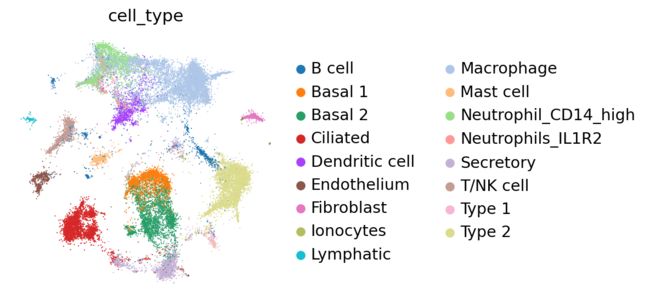
sc.pl.embedding(adata, basis="X_mde", color=["cell_type"], frameon=False, ncols=1)

At a quick glance, it looks like the integration worked well. Indeed, the two datasets are relatively mixed in latent space and the cell types cluster together. We see that this dataset is quite complex, where only some batches contain certain cell types.

scivi整合效果的评价 去除批次效应评价Compute integration metrics

To quantify integration performance, we compute a subset of the metrics from scIB. Note that metrics are manipulated/scaled so that higher is always better, and these metrics might not represent the same exact value as when they were originally described (e.g., ilisi, clisi in this case).

%%capture
def compute_scib_metrics(adata, emb_key, label_key, batch_key, model_name):
    from scib.metrics.silhouette import silhouette_batch, silhouette
    from scib.metrics.lisi import lisi_graph
    import pandas as pd

    emb_key_ = "X_emb"
    adata.obsm[emb_key_] = adata.obsm[emb_key]
    sc.pp.neighbors(adata, use_rep=emb_key_)
    df = pd.DataFrame(index=[model_name])
    df["ilisi"], df["clisi"] = lisi_graph(adata, batch_key, label_key, type_="embed")
    df["sil_batch"] = silhouette_batch(adata, batch_key, label_key, emb_key_)
    df["sil_labels"] = silhouette(adata, label_key, emb_key_)

    return df

emb_key = "X_scVI"
scvi_metrics = compute_scib_metrics(adata, emb_key, "cell_type", "batch", "scVI")
scvi_metrics

Integration with scANVI 如果已经有了细胞注释 scvi如何进行批次矫正 这样的矫正结果更利于轨迹推断

Previously, we used scVI as we assumed we did not have any cell type annotations available to guide us. Consequently, after the previous analysis, one would have to annotate clusters using differential expression, or by other means.

Now, we assume that all of our data is annotated. This can lead to a more accurate integration result when using scANVI, i.e., our latent data manifold is better suited to downstream tasks like visualization, trajectory inference, or nearest-neighbor-based tasks. scANVI requires:

• the sample identifier for each cell (as in scVI)

• the cell type/state for each cell

scANVI can also be used for label transfer and we recommend checking out the other scANVI tutorials to see explore this functionality.

Since we’ve already trained an scVI model on our data, we will use it to initialize scANVI. When initializing scANVI, we provide it the labels_key. As scANVI can also be used for datasets with partially-observed annotations, we need to give it the name of the category that corresponds to unlabeled cells. As we have no unlabeled cells, we can give it any random name that is not the name of an exisiting cell type.

数据输入数据要求Important

scANVI should be initialized from a scVI model pre-trained on the same exact data.

lvae = scvi.model.SCANVI.from_scvi_model(
    vae,
    adata=adata,
    labels_key="cell_type",
    unlabeled_category="Unknown",
)
lvae.train(max_epochs=20, n_samples_per_label=100)

INFO     Training for 20 epochs.

Epoch 20/20: 100%|██████████| 20/20 [01:39<00:00,  4.96s/it, loss=628, v_num=1]

Now we can retrieve the latent space

adata.obsm["X_scANVI"] = lvae.get_latent_representation(adata)

Again, we may visualize the latent space as well as the inferred labels

adata.obsm["X_mde_scanvi"] = mde(adata.obsm["X_scANVI"])
sc.pl.embedding(adata, basis="X_mde_scanvi", color=["cell_type"], ncols=1, frameon=False)