ts12_2Multi-step Forecast_sktime_KNeighbors_WindowSplitter_ForecastingGridSearchCV_exog_EnsembleFore
ts12_Multi-step Forecast_sktime_bold_Linear Regress_sMAPE MASE_warn_plotly acf vlines_season_summary : ts12_Multi-step Forecast_sktime_bold_Linear Regress_sMAPE MASE_warn_plotly acf vlines_season_summary_LIQING LIN的博客-CSDN博客
Optimizing a forecasting model with hyperparameter tuning
You trained different regression models using default parameter values in the previous recipe. A common term for such parameters is hyperparameters, as these are not learned by the model but instead supplied by the user, influencing the model's architecture and behavior.
In this recipe, you will examine how you can find optimal hyperparameter values for the KNN Regresssor (from the previous recipe). You will perform a cross-validated grid search using sktime's ForecastingGridSearchCV.
You have performed a grid search in the Forecasting univariate time series data with non-seasonal ARIMA recipe from ts10_Univariate TS模型_circle mark pAcf_ETS_unpack product_darts_bokeh band interval_ljungbox_AIC_BIC_LIQING LIN的博客-CSDN博客, Building Univariate Time Series Models Using Statistical Methods. Similarly, you were introduced to different automated methods for finding optimal hyperparameters in auto_arima under the Forecasting time series data using auto_arima recipe in ts11_pmdarima_edgecolor_bokeh plotly_Prophet_Fourier_VAR_endog exog_Granger causality_IRF_Garch vola_LIQING LIN的博客-CSDN博客, Additional Statistical Modeling Techniques for Time Series.
You will load the same libraries from the previous recipe, Multi-step forecasting using linear regression models with scikit-learn. The following are the additional classes and functions you will need for this recipe.
You will import the three classes, ForecastingGridSearchCV, SlidingWindowSplitter, and MeanAbsolutePercentageError. The metric class will be used in the cross-validated grid search for evaluating the different models, but you could use any other metric:
from sktime.forecasting.all import ( ForecastingGridSearchCV,
                                     SlidingWindowSplitter,
                                     MeanSquaredPercentageError
                                   )
df_energy = energy.copy(deep=True)
df_energy
You will build a K-NN regression model based on the results from the previous recipe, and then work on optimizing the model with hyperparameter tuning. The following steps will use the energy DataFrame, but you should be able to apply the same steps on the other two datasets:
1. Make a copy of the energy DataFrame and split the data into training and test sets:

# def split_data( df, test_split=0.15 ):
#     n = int( len(df) * test_split )
#     train, test = df[:-n], df[-n:]
#     return train, test

train_energy, test_energy = split_data(df_energy)
train_energy

2. You will use the TransformedTargetForecaster class to create a pipeline for transforming the time series:
from sktime.forecasting.all import ( NaiveForecaster,
                                     Deseasonalizer, Detrender,
                                     temporal_train_test_split,
                                     mean_absolute_percentage_error as mape,
                                     mean_squared_percentage_error as mspe,
                                     mean_squared_error as mse,
                                     ForecastingHorizon,
                                     TransformedTargetForecaster,
                                     PolynomialTrendForecaster
                                   )
from sktime.forecasting.compose import make_reduction
from sklearn.neighbors import KNeighborsRegressor

n = len(test_energy)
fh = ForecastingHorizon( np.arange(n)+1,
                         is_relative=True
                       )# True: forecasting horizon is relative to the end of the training series
forecaster = TransformedTargetForecaster( [('deseasonalize',
                                            Deseasonalizer( model='multiplicative', sp=12)
                                           ),
                                           ('detrend',
                                            Detrender( forecaster=PolynomialTrendForecaster(degree=1) )
                                           ),
                                           ('forecast',
                                            make_reduction( KNeighborsRegressor(),
                                                            scitype='tabular-regressor',
                                                            window_length=12,
                                                            strategy='recursive',
                                                          )
                                           ),
                                          ] )
forecaster
Notice the use of the make_reduction function in the pipeline before fitting (training) the model. This will create a reduced regression for the time series data. You will learn more on the concept of a reduced form in the How it works... section. For now, realize that make_reduction will return a RecursiveTabularRegressionForecaster class, and the default strategy parameter is recursive.

Train the model using the fit method and store the predictions as a new column in the test DataFrame using the predict method:
forecaster.fit( train_energy.values )
test_energy['KNN-Regressor'] = forecaster.predict( fh )
test_energy 
3. You will use the evaluate function created in the preceding Multi-step forecasting using linear regression models with scikit-learn recipe to evaluate the model:
from sktime.performance_metrics.forecasting import( MeanSquaredError,
                                                    MeanAbsolutePercentageError,
                                                    MeanAbsoluteScaledError
                                                  )
mse = MeanSquaredError()
mape = MeanAbsolutePercentageError()
mase = MeanAbsoluteScaledError()

def evaluate( df, train, sort_by = 'MASE'):
    evals = pd.DataFrame( index=['sMAPE', 'MAPE', 'RMSE'] )
    y_truth = df['y']
    y_predicted = df.drop( columns=['y'] )
    for p in y_predicted:
        evals.loc['sMAPE', p] = mape( y_truth, y_predicted[p], symmetric=True )
        evals.loc['MAPE', p] = mape( y_truth, y_predicted[p], symmetric=False )
        evals.loc['RMSE', p] = np.sqrt( mse(y_truth, y_predicted[p]) )
        evals.loc['MASE', p] = mase( y_truth, y_predicted[p], y_train=train )
    return evals.T.sort_values(by=sort_by)

evaluate( test_energy, train_energy ) ![]()
4. Inspect the parameters available from the forecaster object with the get_params method. The following shows a small subset of the output:
forecaster.get_params() The output shows the available hyperparameters that you can control.
forecaster.get_params().keys()
5. Create a Python dictionary to define the hyperparameters you want to optimize against. The following is an example:
hyperparams_grid = { 'forecast__estimator__n_neighbors': [ i for i in range(3,11) ], # for knn
                     'deseasonalize__model': ['multiplicative', 'additive'],
                     'forecast__estimator__p':[1,2] # Power parameter for the Minkowski metric.
                   }# When p = 1, this is equivalent to using manhattan_distance (l1),
                    # and euclidean_distance (l2) for p = 2
In the preceding code, there are three hyperparameters with a range of values to evaluate against. In grid search, at every iteration, a model is trained and evaluated using a different combination of values until all combinations have been evaluated. When using ForecastingGridSearchCV, you can specify a metric to use for evaluating the models, for example, scoring=smape.
######################
SlidingWindowSplitter — sktime documentation
class SlidingWindowSplitter(fh: Union[int,
                                      list,
                                      numpy.ndarray,
                                      pandas.core.indexes.base.Index,
                                      sktime.forecasting.base._fh.ForecastingHorizon
                                     ] = 1,
                            window_length: Union[int,
                                                 float,
                                                 pandas._libs.tslibs.timedeltas.Timedelta,
                                                 datetime.timedelta,
                                                 numpy.timedelta64,
                                                 pandas._libs.tslibs.offsets.DateOffset
                                                ] = 10,
                            step_length: Union[int,
                                               pandas._libs.tslibs.timedeltas.Timedelta,
                                               datetime.timedelta,
                                               numpy.timedelta64,
                                               pandas._libs.tslibs.offsets.DateOffset
                                              ] = 1,
                            initial_window: Optional[Union[int,
                                                           float,
                                                   pandas._libs.tslibs.timedeltas.Timedelta,
                                                           datetime.timedelta,
                                                           numpy.timedelta64,
                                                           pandas._libs.tslibs.offsets.DateOffset
                                                          ]
                                                    ] = None,
                            start_with_window: bool = True
                           )
Sliding window splitter.
Split time series repeatedly into a fixed-length training and test set.
It is required that the window length plus maximum forecast horizon is smaller than the length of the time series `y` itself. : len(df_energy)*0.70 + fh < len(train_energy) please see follow steps.
Test window is defined by forecasting horizons relative to the end of the training window. It will contain as many indices as there are forecasting horizons provided to the fh argument. For a forecasating horizon (![]() ,…,
,…,![]() ),
),
the training window will consist of the indices (![]() ,…,
,…,![]() ).
).
For example for window_length = 5, step_length = 1 and fh = [1, 2, 3] here is a representation of the folds:
|----------------------->
| * * * * * x x x - - - >
| - * * * * * x x x - - >
| - - * * * * * x x x - >
| - - - * * * * * x x x >
* = training fold.
x = test fold.
Parameters
fh int, list or np.array
Forecasting horizon
window_length int or timedelta or pd.DateOffset
Window length
step_length int or timedelta or pd.DateOffset, optional (default=1)
Step length between windows
initial_window int or timedelta or pd.DateOffset, optional (default=None)
Window length of first window
start_with_window bool, optional (default=True)
-
If True, starts with full window.
-
If False, starts with empty window.
ForecastingGridSearchCV — sktime documentation
class ForecastingGridSearchCV(forecaster, cv, param_grid, scoring=None,
                              strategy='refit', n_jobs=None, refit=True,
                              verbose=0, return_n_best_forecasters=1,
                              pre_dispatch='2*n_jobs', backend='loky',
                              update_behaviour='full_refit', error_score=nan
                             )
Perform grid-search cross-validation to find optimal model parameters.
The forecaster is fit on the initial window and then temporal cross-validation is used to find the optimal parameter.
Grid-search cross-validation is performed based on a cross-validation iterator encoding the cross-validation scheme, the parameter grid to search over, and (optionally) the evaluation metric for comparing model performance. As in scikit-learn, tuning works through the common hyper-parameter interface which allows to repeatedly fit and evaluate the same forecaster with different hyper-parameters.
Parameters
forecaster estimator object
The estimator should implement the sktime or scikit-learn estimator interface. Either the estimator must contain a “score” function, or a scoring function must be passed.
cv cross-validation generator or an iterable
e.g. SlidingWindowSplitter()
strategy {“refit”, “update”, “no-update_params”}, optional, default=”refit”
data ingestion strategy in fitting cv, passed to evaluate internally defines the ingestion mode when the forecaster sees new data when window expands
- “refit” = forecaster is refitted to each training window
- “update” = forecaster is updated with training window data, in sequence provided按提供的顺序更新训练窗口数据
- “no-update_params” = fit to first training window, re-used without fit or update
update_behaviour: str, optional, default = “full_refit”
one of {“full_refit”, “inner_only”, “no_update”} behaviour of the forecaster when calling update “full_refit” = both tuning parameters and inner estimator refit on all data seen
“inner_only” = tuning parameters are not re-tuned, inner estimator is updated
“no_update” = neither tuning parameters nor inner estimator are updated
param_grid dict or list of dictionaries
Model tuning parameters of the forecaster to evaluate
scoring: function, optional (default=None)
Function to score models for evaluation of optimal parameters
n_jobs: int, optional (default=None)
Number of jobs to run in parallel.
- None means 1 unless in a joblib.parallel_backend context.
- -1 means using all processors.
refit: bool, optional (default=True)
- True = refit the forecaster with the best parameters on the entire data in fit
- False = best forecaster remains fitted on the last fold in cv
verbose: int, optional (default=0)
verbose is set to 1 to print a summary for the number of computations.
The default is verbose=0 , which will not print anything.
return_n_best_forecasters: int, default=1
In case the n best forecaster should be returned, this value can be set and the n best forecasters will be assigned to n_best_forecasters_
pre_dispatch: str, optional (default=’2*n_jobs’)
error_score: numeric value or the str ‘raise’, optional (default=np.nan)
The test score returned when a forecaster fails to be fitted.
Value to assign to the score if an exception occurs in estimator fitting.
If set to “raise”, the exception is raised.
If a numeric value is given, FitFailedWarning is raised.
return_train_score: bool, optional (default=False)
backend: str, optional (default=”loky”)
Specify the parallelisation backend implementation in joblib, where “loky” is used by default.
Attributes
best_index_ int
best_score_: float
Score of the best model
best_params_dict
Best parameter values across the parameter grid
best_forecaster_estimator
Fitted estimator with the best parameters
cv_results_ dict
Results from grid search cross validation
n_splits_: int
Number of splits in the data for cross validation
refit_time_ float
Time (seconds) to refit the best forecaster
scorer_ function
Function used to score model
n_best_forecasters_: list of tuples (“rank”,
The “rank” is in relation to best_forecaster_
n_best_scores_: list of float
The scores of n_best_forecasters_ sorted from best to worst score of forecasters
######################
6. To perform cross-validation on time series, you will use the SlidingWindowSplitter class and define a sliding window at 70% of the df DataFrame (notice you are not using the train DataFrame). This means that 70% of the data will be allocated for the training fold and while the testing fold based on fh , or forecast horizon.
It is required that the window length plus maximum forecast horizon is smaller than the length of the time series `y` itself: len(df_energy)*0.70 + fh < len(train_energy).
cp6_Model Eval_Confusion_Hyperpara Tuning_pipeline_variance_bias_ validation_learning curve_strength_LIQING LIN的博客-CSDN博客Create the grid search object grid_scv using the ForecastingGridSearchCV class:
cv = SlidingWindowSplitter( window_length=int( len(df_energy)*0.70 ),#0.7 training set,0.3 test set
                            fh=fh                                    #len(df_energy)*0.70 + fh < len(train_energy)
                          )
smape = MeanAbsolutePercentageError( symmetric=True )
sktime
Currently, sktime only supports grid search and random search.
grid_scv = ForecastingGridSearchCV( forecaster,
                                    strategy='refit', # forecaster is refitted to each training window
                                    cv=cv,
                                    param_grid=hyperparams_grid,
                                    scoring=smape,
                                    return_n_best_forecasters=1,
                                    verbose=1
                                  )
Notice that verbose is set to 1 to print a summary for the number of computations. The default is verbose=0 , which will not print anything.
grid_scv.cv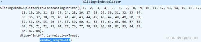
7. To initiate the process and train the different models, use the fit method:
grid_scv.fit(train_energy.values, fh=fh)


The following output is based on the 8 hyperparameters listed earlier:
![]()
The total number of models to be evaluated is 64 .
It is required that the window length plus maximum forecast horizon is smaller than the length of the time series `y` itself: len(df_energy)*0.70 + fh < len(train_energy).
window_length : len(df_energy)*0.7
The cross-validated process produced 2 folds(
2 steps(folds) = len(train_energy)- len(df_energy)*0.7 + fh +1 =500-411-88 +1=2
32 steps(folds) =len(df_energy[:int(-len(df_energy)*0.1)]) - len(df_energy)*0.7 + fh +1 =530-411-88 +1=32
). There are 32 total combinations ( 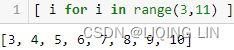
 n_neighbors(8) X seasonality(2) X P(2) = 32) . The total number of models that will be trained ( fit ) is 2 x 32 = 64 . Alternatively, you could use ForecastingRandomizedSearchCV , which performs a randomized cross-validated grid search to find optimal hyperparameters and is generally faster, but there is still a random component to the process.
Changing the number of folds can be controlled using window_length from the SlidingWindowSplitter class, which was set at 70% of the data.
8. Once the grid search process is completed, you can access the list of optimal hyperparameters using the best_params attribute.:
grid_scv.best_params_ 
grid_scv.best_forecaster_
9. You can use the predict method from the grid_scv object to produce a forecast. Store the results as a new column in the test DataFrame to compare the results from the optimized hyperparameters against the default values used earlier in the recipe:
test_energy['KNN_optimized'] = grid_scv.predict(fh)
test_energy 
Use the evaluate function to compare the two results:
evaluate(test_energy, train_energy)This should produce a DataFrame comparing the two models, RandomForestRegressor and RandomForestRegressor_optim , that looks like this:

Figure 12.13 – Scores of an optimized KNN regressor and standard KNN regressor
Overall, the optimized K-NN regression did outperform the standard model with default values.
test_energy.plot()
plt.show()
The sktime library provides three splitting options for cross-validation:
- SingleWindowSplitter,
The SingleWindowSplitter class splits the data into training and test sets only once. - SlidingWindowSplitter, and
- ExpandingWindowSplitter .
The difference between the sliding and expanding splitters is how the training fold size changes. This is better explained through the following diagram:  Figure 12.14 – Difference between SlidingWindowSplitter and ExpandingWindowSplitter
Notice from Figure 12.14 that
- SlidingWindowSplitter, as the name implies, just slides over one step at each iteration, keeping the training and test fold(fh) sizes constant.
- In the ExpandingWindowSplitter, the training fold expands by one step at each iteration.
The step size behavior can be adjusted using the step_length parameter (default is 1). Each row in Figure 12.14 represents a model that is being trained (fitted) on the designated training fold and evaluated against the designated testing fold(fh). After the entire run is complete the mean score is calculated.
To get more insight into the performance at each fold, you can use the cv_results_ attribute. This should produce a DataFrame of 32 rows, one row for each of the 32 combinations
( n_neighbors(8) X seasonality(2) X P(2) = 32)
), and the mean scores are for the 2 folds(
2 steps(folds) = len(train_energy)- len(df_energy)*0.7 + fh +1 =500-411-88 +1=2
):
grid_scv.cv_results_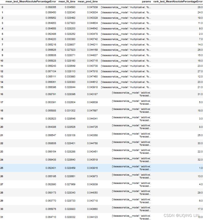
The preceding code will return a DataFrame showing the average scores of all the folds for each combination (model).
And if you want to store the model or see the full list of parameters, you can use the best_forecaster_ attribute:
model_KNN_optimized = grid_scv.best_forecaster_
model_KNN_optimized.get_params()
This should list all the parameters available and their values.
You can learn more about the ForecastingGridSearchCV class from the official documentation at ForecastingGridSearchCV — sktime documentation.
Forecasting with exogenous variables and ensemble learning
This recipe will allow you to explore two different techniques: working with multivariate time series and using ensemble forecasters. For example, the EnsembleForecaster class takes in a list of multiple regressors, each regressor gets trained, and collectively contribute in making a prediction. This is accomplished by taking the average of the individual predictions from each regressor. Think of this as the power of the collective. You will use the same regressors you used earlier: Linear Regression, Random Forest Regressor, Gradient Boosting Regressor, and Support Vector Machines Regressor.
You will use a Naive Regressor as the baseline to compare with EnsembleForecaster. Additionally, you will use exogenous variables with the Ensemble Forecaster to model a multivariate time series. You can use any regressor that accepts exogenous variables.
You will load the same modules and libraries from the previous recipe, Multi-step forecasting using linear regression models with scikit-learn. The following are the additional classes and functions you will need for this recipe:
from sktime.forecasting.all import EnsembleForecaster
from sklearn.svm import SVR
from sktime.transformations.series.detrend import ConditionalDeseasonalizer
from sktime.datasets import load_macroeconomic
1. Load the macroeconomic data, which contains 12 features:
econ = load_macroeconomic()
econ
cols = ['realgdp','realdpi','tbilrate', 'unemp', 'infl']
econ_df = econ[cols]

econ_df.plot( subplots=True, figsize=(16,10) )
plt.show()
You want to predict the unemployment rate (unemp) using exogenous variables. The exogenous variables include
- real gross domestic product (realgpd)实际国内生产总值,
- real disposable personal income (realdpi)实际可支配个人收入,
- the Treasury bill rate (tbilrate)国库券利率,
- and inflation (infl)通货膨胀.
This is similar to univariate time series forecasting with exogenous variables(independent variables)外生变量. This is different from the VAR model which is used with multivariate time seriests11_pmdarima_edgecolor_bokeh plotly_Prophet_Fourier_VAR_endog exog_Granger causality_IRF_Garch vola_LIQING LIN的博客-CSDN博客and treats the variables as endogenous variables(dependent variables, Endogenous variables are influenced by other variables within the system)内生变量.
2. The reference for the endogenous, or univariate, variable in sktime is y and X for the exogenous variables. Split the data into y_train, y_test , exog_train, and exog_test :
y = econ_df['unemp']
exog = econ_df.drop( columns=['unemp'] )

test_size = 0.1
y_train, y_test = split_data( y, test_split=test_size )
exog_train, exog_test = split_data( exog, test_split=test_size )
exog_train

 Time Series / Date functionality — pandas 0.13.1 documentation

exog_test 
3. Create a list of the regressors to be used with EnsembleForecaster :
###############
make_reduction(estimator, strategy='recursive', window_length=10,
               scitype='infer', transformers=None, pooling='local'
              )
Make forecaster based on reduction to tabular or time-series regression.
During fitting, a sliding-window approach is used to first transform the time series into tabular or panel data, which is then used to fit a tabular or time-series regression estimator. During prediction, the last available data is used as input to the fitted regression estimator to generate forecasts. https://blog.csdn.net/Linli522362242/article/details/128506988
###############
regressors = [( 'LinearRegression', make_reduction( LinearRegression() ) ),
              ( 'RandomForest', make_reduction( RandomForestRegressor() ) ),
              ( 'SupportVectorRegressor', make_reduction( SVR() ) ),
              ( 'GradientBoosting', make_reduction( GradientBoostingRegressor() ) )
             ]
4. Create an instance of the EnsembleForecaster class and the NaiveForecaster() class with default hyperparameter values.
ensemble = EnsembleForecaster( regressors )
naive = NaiveForecaster()
5. Train both forecasters on the training set with the fit method. You will supply the univariate time series (y) along with the exogenous variables (X):
ensemble.fit( y=y_train, X=exog_train )
naive.fit( y=y_train, X=exog_train )![]()
6. Once training is complete, you can use the predict method, supplying the forecast horizon and the test exogenous variables. This will be the unseen exog_test set:
y_test 
fh = ForecastingHorizon( y_test.index, is_relative=None ) #None:the flag is determined automatically

y_hat = pd.DataFrame( y_test ).rename( columns={'unemp': 'test'} )
y_hat['EnsembleForecaster'] = ensemble.predict( fh=fh, X=exog_test )
y_hat['NaiveForecaster'] = naive.predict( fh=fh, X=exog_test )
y_hat.rename( columns={'test':'y'}, inplace=True )

y_hat 
7. Use the evaluate function that you created earlier in the Forecasting using non-linear models with sktime recipe:
evaluate( y_hat, y_train )
Figure 12.15 – Evaluation of NaiveForecaster and EnsembleForecaster
Overall, EnsembleForecaster did better than NaiveForecaster.
You can plot both forecasters for a visual comparison as well:
styles = ['k--', 'bx-', 'yv-']
for col, s in zip( y_hat, styles ):
    y_hat[col].plot( style=s, label=col,
                     title=r'$\bfEnsembleForecaster$ vs $\bfNaiveForecaster$',
                     figsize=(10,6)
                   )
plt.legend()
plt.show()
The preceding code should produce a plot showing all three time series for EnsembleForecaster, NaiveForecaster, and the test dataset.
Figure 12.16 – Plotting the three forecasters against the test data
Remember that neither of the models was optimized. Ideally, you can use k-fold cross-validation when training or a cross-validated grid search, as shown in the Optimizing a forecasting model with hyperparameter tuning recipe.
The EnsembleForecaster class from sktime is similar to the VotingRegressor class in sklearn. Both are ensemble estimators that fit (train) several regressors and collectively, they produce a prediction through an aggregate function. Unlike VotingRegressor in sklearn, EnsembleForecaster allows you to change the aggfunc parameter to either mean (default), median, min, or max. When making a prediction with the predict method, only one prediction per one-step forecast horizon is produced. In other words, you will not get multiple predictions from each base regressor, but rather the aggregated value (for example, the mean) from all the base regressors.
Using a multivariate time series is made simple by using exogenous variables. Similarly, in statsmodels , an ARIMA or SARIMA model has an exog parameter. An ARIMA with exogenous variables is referred to as ARIMAX. Similarly, a seasonal ARIMA with exogenous variables is referred to as SARIMAX. To learn more about exogenous variables in statsmodels, you can refer to the documentation here: endog, exog, what’s that? — statsmodels.
class AutoEnsembleForecaster(forecasters, regressor=None, test_size=None,
                             random_state=None, n_jobs=None
                            )
Automatically find best weights for the ensembled forecasters.
The AutoEnsembleForecaster uses a meta-model (regressor) to calculate the optimal weights for ensemble aggregation with mean. The regressor has to be sklearn-like and needs to have either an attribute feature_importances_ (07_Ensemble Learning and Random Forests_Bagging_Out-of-Bag_Random Forests_Extra-Trees极端随机树_Boosting_LIQING LIN的博客-CSDN博客) or coef_, as this is used as weights. Regressor can also be a sklearn.Pipeline.
Parameters
forecasters list of (str, estimator) tuples
Estimators to apply to the input series.
regressor sklearn-like regressor, optional, default=None.
Used to infer optimal weights from coefficients (linear models) or from feature importance scores (decision tree-based models). If None, then a GradientBoostingRegressor(max_depth=5) is used. The regressor can also be a sklearn.Pipeline().
test_size int or float, optional, default=None
Used to do an internal temporal_train_test_split(). The test_size data will be the endog data of the regressor and it is the most recent data. The exog data of the regressor are the predictions from the temporarily trained ensemble models. If None, it will be set to 0.25.
random_state int, RandomState instance or None, default=None
Used to set random_state of the default regressor.
n_jobs int or None, optional, default=None
The number of jobs to run in parallel for fit. None means 1 unless in a joblib.parallel_backend context. -1 means using all processors.
Attributes
regressor_ sklearn-like regressor
Fitted regressor.
weights_ np.array
The weights based on either regressor.feature_importances_ or regressor.coef_ values.
The AutoEnsembleForecaster class in sktime behaves similar to the EnsembleForecaster class you used earlier. The difference is that
- the AutoEnsembleForecaster class will calculate the optimal weights for each of the regressors passed.
- The AutoEnsembleForecaster class has a regressor parameter that takes a list of regressors and estimates a weight for each class.
In other words, not all regressors are treated equal.
If none are provided, then the GradientBoostingRegressor class is used instead, with a default max_depth=5. 07_Ensemble Learning and Random Forests_02_AdaBoost_更新Gradient Boosting_XGBoost_LIQING LIN的博客-CSDN博客
Using the same list of regressors, you will use AutoEnsembleForecaster and compare the results with RandomForest and EnsembleForecaster.
regressors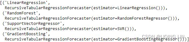
from sktime.forecasting.compose import AutoEnsembleForecaster

auto = AutoEnsembleForecaster( forecasters=regressors,
                               method='feature-importance'
                             )
auto.fit( y=y_train, X=exog_train )
auto.weights_ 
The order of the weights listed are based on the order from the regressor list provided. The highest weight was given to GradientBoostingRegressor at 64% followed by SupportVectorRegressor at 19%.
Using the predict method, let's compare the results:
y_hat['AutoEnsembleForecaster'] = auto.predict( fh=fh, X=exog_test )
y_hat
evaluate( y_hat, y_train ) 
Figure12.17–Evaluation of RandomForest, EnsembleForecaster, and AutoEnsembleForecaster
Keep in mind that the number and type of regressors (or forecasters) used in both EnsembleForecaster and AutoEnsembleForecaster will have a significant impact on the overall quality. Keep in mind that none of these models have been optimized and are based on default hyperparameter values.
To learn more about the AutoEnsembleForecaster class, you can read the official documentation here: AutoEnsembleForecaster — sktime documentation.
To learn more about the EnsembleForecaster class, you can read the official documentation here: EnsembleForecaster — sktime documentation.