为什么要进行时间序列分类?(Why Time Series Classification?)
First of all it’s important to underline why this problem is so important today, and therefore why it is very interesting to understand the role and the potential of Deep Learning in this sector.
首先,重要的是要强调为什么这个问题在今天如此重要,因此为什么理解深度学习在该领域的作用和潜力非常有趣。
During the last years, Time Series Classification has become one of the most challenging problems in Data Science. This has happened because any classification problem that uses data keeping in consideration some notion of sorting, can be treated as a Time Series Classification problem.
在过去的几年中,时间序列分类已成为数据科学中最具挑战性的问题之一。 之所以发生这种情况,是因为考虑到排序的某些概念而使用数据的任何分类问题都可以被视为时间序列分类问题。
Time series are present in many real-world applications ranging from health care, human activity recognition, cyber-security, finance, marketing, automated disease detection, anomaly detection, etc. As the availability of temporal data has increased significantly in the last years, many areas are becoming strongly interested in applications based on time series, and then many new algorithms have been proposed.
时间序列存在于许多实际应用中,包括医疗保健,人类活动识别,网络安全,金融,市场营销,自动疾病检测,异常检测等。随着近几年时间数据的可用性显着增加,许多领域都对基于时间序列的应用程序产生了浓厚的兴趣,然后提出了许多新算法。
All these algorithms, apart from those based on deep learning, require some kind of feature engineering as a separate task before the classification is performed, and this can imply the loss of some information and the increase of the development time. On the contrary, deep learning models already incorporate this kind of feature engineering internally, optimizing it and eliminating the need to do it manually. Therefore they are able to extract information from the time series in a faster, more direct, and more complete way.
除了基于深度学习的算法以外,所有这些算法在进行分类之前都需要某种特征工程作为单独的任务,这可能意味着某些信息的丢失和开发时间的增加。 相反,深度学习模型已经在内部合并了此类功能工程,从而对其进行了优化并消除了手动进行操作的需要。 因此,他们能够以更快,更直接,更完整的方式从时间序列中提取信息。
应用领域 (Applications)
Let’s see some important applications of Reinforcement Learning.
让我们看看强化学习的一些重要应用。
Electrocardiogram records can be used to find out various heart problems, and are saved in time series form. Distinguishing the electrocardiogram of a normal heart from the one of a heart with a disease, and recognizing the disease, is a Time Series Classification problem.
心电图记录可用于发现各种心脏问题,并以时间序列形式保存。 将正常心脏的心电图与患有疾病的心脏的心电图区分开并识别疾病是时间序列分类问题。
Today many devices can be controlled with the use of simple gestures, without physically touching them. For this purpose these devices record a series of images that are used to interpret the user’s gestures. Identifying the correct gesture from this sequence of images is a Time SeriesClassification problem. Anomaly detection is the identification of unusual events or observations which are significantly different from the majority of the data.
如今,许多设备都可以使用简单的手势进行控制,而无需实际触摸它们。 为此,这些设备记录了一系列图像,这些图像用于解释用户的手势。 从图像序列中识别正确的手势是一个时间序列分类问题。 异常检测是对与大多数数据有显着差异的异常事件或观察结果的识别。
Often the data in anomaly detection are time series, for example the temporal trend of a magnitude related to an electronic device, monitored to check that the device is working correctly. Distinguishing the time series of normal operations from that of a device with some anomaly, and recognizing the anomaly, is a Time Series Classification problem.
异常检测中的数据通常是时间序列,例如与电子设备相关的幅度的时间趋势,需要对其进行监视以检查设备是否正常工作。 将正常操作的时间序列与具有某些异常的设备的时间序列区分开,并识别异常是时间序列分类问题。
问题定义 (Problem definition)
Now we give a formal definition of a Time Series Classification problem. Suppose to have a set of objects with the same structure (for example real values, vectors or matrices with same size, etc.), and a fixed set of different classes. We define a dataset as a collection of pairs (object, class), which means that to each object is associated a determinate class. Given a dataset, a Classification problem is building a model that associates to a new object, with the same structure of the others, the probability to belong to the possible classes, accordingly to the features of the objects associated to each class.
现在我们给出时间序列分类问题的正式定义。 假设有一组具有相同结构的对象(例如,具有相同大小的实数值,向量或矩阵等),以及一组固定的不同类。 我们将数据集定义为对(对象,类)对的集合,这意味着每个对象都关联有一个确定的类。 给定一个数据集,分类问题正在建立一个模型,该模型与一个新对象相关联,并且具有与其他对象相同的结构,从而根据与每个类相关联的对象的特征,属于可能类的可能性。
An univariate time series is an ordered set of real values, while a M dimensional multivariate time series consists of M different univariate time series with the same length. A Time Series Classification problem is a Classification problem where the objects of the dataset are univariate or multivariate time series.
单变量时间序列是有序的实数值集,而M维多元时间序列由M个长度相同的不同单变量时间序列组成。 时间序列分类问题是一个分类问题,其中数据集的对象是单变量或多变量时间序列。
感知器(神经元) (Perceptron (Neuron))
Before introducing the different types of Deep Learning Architectures, we recall some basic structures that they use. First of all we introduce the Perceptron, that is the basic element of many machine learning algorithms. It is inspired by the functionality of biological neural circuits, and for this reason is also called neuron.
在介绍不同类型的深度学习架构之前,我们回顾一下它们使用的一些基本结构。 首先,我们介绍Perceptron,这是许多机器学习算法的基本要素。 它受到生物神经回路功能的启发,因此也称为神经元。
This Figure shows the architecture of a Perceptron. A Perceptron has one or more input values, and every input value is associated to a weight.
该图显示了感知器的体系结构。 感知器具有一个或多个输入值,并且每个输入值都与一个权重相关联。
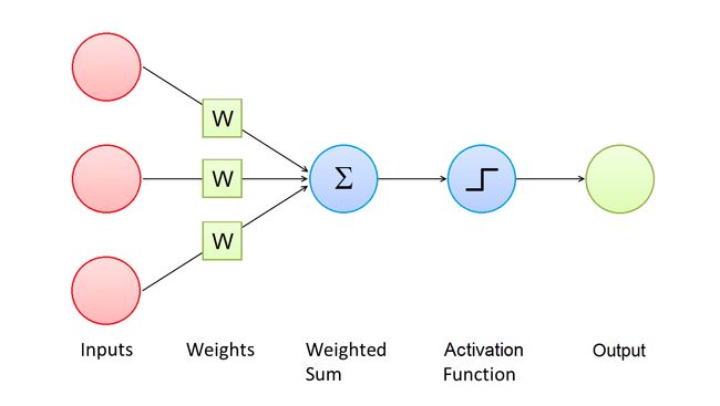
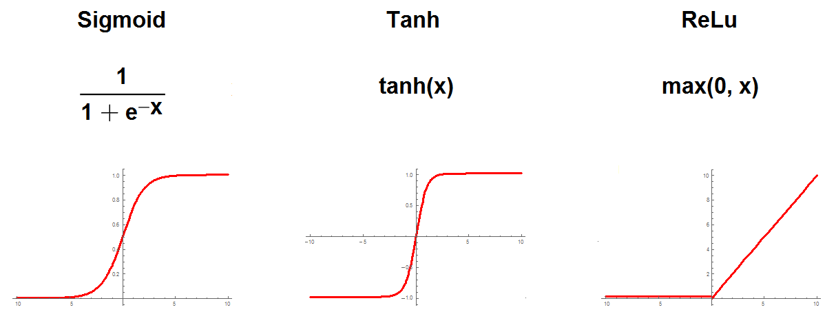
The goal of a Perceptron is to compute the wighted sum of the input values and then apply an activation function to the result. The most common activation functions are sigmoid, hyperbolic tangent and rectifier:
感知器的目标是计算输入值的加权总和,然后将激活函数应用于结果。 最常见的激活函数是S型,双曲正切和整流器:
The result of the activation function is referred as the activation of the Perceptron and represents its output value.
激活功能的结果称为感知器的激活,并表示其输出值。
多层感知器 (Multi Layer Perceptron)
Now we introduce the Multi Layer Perceptron (MLP), that is a building block used in many Deep Learning Architectures for Time Series Classification. It is a class of feedforward neural networks and consists of several layers of nodes: one input layer, one or more hidden layers, and one output layer. Every node is connected to all the nodes of its layer, of the previous layer and of the next layer. For this reason we say that Multi Layer Perceptron is fully connected. Each node of the hidden layers and of the output layer is a Perceptron.
现在,我们介绍多层感知器(MLP),它是许多用于时间序列分类的深度学习架构中使用的构建块。 它是一类前馈神经网络,由几层节点组成:一个输入层,一个或多个隐藏层以及一个输出层。 每个节点都连接到其层,上一层和下一层的所有节点。 因此,我们说多层感知器已完全连接。 隐藏层和输出层的每个节点都是一个感知器。
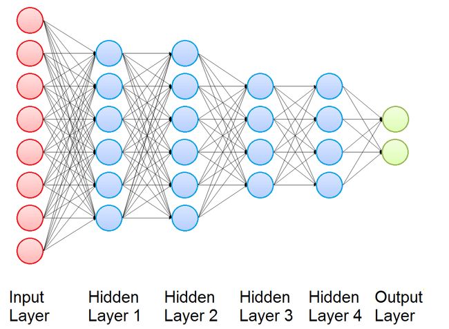
The output of the Multi Layer Perceptron is obtained computing in sequence the activation of its Perceptrons, and the function that connect the input and the output depends on the values of the weights.
多层感知器的输出是通过依次计算其感知器的激活而获得的,连接输入和输出的功能取决于权重的值。
多层感知器分类 (Classification with Multi Layer Perceptron)
Multi Layer Perceptron is commonly used for Classification problems: given a dataset (that we recall to be a collection of pairs (object, class)), it can be fitted to compute the probability of any new object to belong to each possible class. To do this, first of all we need to represent the pairs (object, class) in the dataset in a more suitable way:
多层感知器通常用于分类问题:给定一个数据集(我们记得它是对(对象,类)的集合),它可以适合计算任何新对象属于每个可能类的概率。 为此,首先我们需要以更合适的方式在数据集中表示对(对象,类):
- Every object must be flattened and then represented with a vector, that will be the input vector for training. 必须将每个对象弄平,然后用向量表示,该向量将作为训练的输入向量。
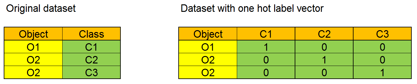
Every class in the dataset must be represented with its one-hot label vector. A one-hot label vector is a vector with size equal to the number of different classes in the dataset. Each element of the array corresponds to a possible class, and every value is 0 apart from that related to the represented class, that is 1. The one-hot label vector will be the target for training. We can see a simple exampe of one hot label vector in this Figure: in the original dataset the column Class has three different values, and the dataset with the one hot label vector has three columns, one for each class.
数据集中的每个类都必须用其一号标签向量表示。 一键式标签向量是大小等于数据集中不同类的数量的向量。 数组的每个元素对应于一个可能的类,并且每个值除与表示的类相关的值外均为0 ,即1 。 一站式标签向量将成为训练的目标。 我们可以在此图中看到一个热标签向量的简单示例:在原始数据集中,列Class具有三个不同的值,而具有一个热标签向量的数据集具有三列,每个列对应一个。
In this way we obtain a new dataset of pairs (input vector, target), and we are ready for training. For this process, MLP uses a supervised learning technique called Backpropagation, that works iterating on the input vectors of the dataset:
这样,我们获得了一个新的对数据集(输入向量,目标),并且已经准备好进行训练。 对于此过程,MLP使用一种称为反向传播的监督学习技术,该技术可对数据集的输入向量进行迭代:
- At every iteration, the output of the Mlp is computed using the present input vector. 在每次迭代中,使用当前输入向量计算Mlp的输出。
- The output is a vector whose components are the estimated probabilities of belonging to each class. 输出是一个向量,向量的组成部分是属于每个类别的估计概率。
- The model’s prediction error is computed using a cost function. 使用成本函数计算模型的预测误差。
- Then, using gradient descent, the weights are updated in a backward pass to propagate the error. 然后,使用梯度下降,权重在向后传递中更新以传播误差。
Thus, by iteratively taking a forward pass followed by backpropagation, the model’s weights are updated in a way that minimizes the loss on the training data. After the training, when the input of the Multi Layer Perceptron is the vector corresponding to an object with the given structure, also not present in the dataset, the output is a vector whose components are the estimated probabilities of belonging to each class.
因此,通过反复进行前向传播和反向传播,可以以最小化训练数据损失的方式更新模型的权重。 训练后,当多层感知器的输入是与具有给定结构的对象相对应的向量(数据集中也没有出现)时,输出是一个向量,其分量是属于每个类别的估计概率。
Now, the natural question is: why don’t use the Multi Layer Perceptron for Time Series Classification, taking the whole multivariate time series as input? The answer is that Multi Layer Perceptron, as many other Machine Learning algorithms, don’t work well for Time Series Classification because the length of the time series really hurts the computational speed. Hence, to obtain good results for Time Series Classification it is necessary to extract the relevant features of the input time series, and use them as input of a classification algorithm, in order to obtain better results in a very lower computation time.
现在,自然的问题是:为什么不使用多层感知器进行时间序列分类,而将整个多元时间序列作为输入呢? 答案是,与许多其他机器学习算法一样,多层感知器不适用于时间序列分类,因为时间序列的长度确实会损害计算速度。 因此,为了获得时间序列分类的良好结果,有必要提取输入时间序列的相关特征,并将其用作分类算法的输入,以便在非常短的计算时间内获得更好的结果。
The big advantage of Deep Learning algorithms with respect to other algorithms is that these relevant feature are learned during the training, and not handcrafted. This improves very much the accuracy of the results and makes the data preparation time much lower. Then, after many layers used for the extraction of these relevant features, many Deep Learning architecures can use algorithms like MLP to obtain the desired classification.
深度学习算法相对于其他算法的最大优势是,这些相关功能是在训练期间学习的,而不是手工制作的。 这极大地提高了结果的准确性,并使数据准备时间大大缩短。 然后,在用于提取这些相关特征的许多层之后,许多深度学习架构可以使用诸如MLP之类的算法来获得所需的分类。
时间序列分类的深度学习 (Deep Learning for Time Series Classification)

This Figure shows a general Deep Learning framework for Time Series Classification. It is a composition of several layers that implement non-linear functions. The input is a multivariate time series. Every layer takes as input the output of the previous layer and applies its non-linear transformation to compute its own output.
该图显示了用于时间序列分类的通用深度学习框架。 它由实现非线性功能的几层组成。 输入是一个多元时间序列。 每层都将上一层的输出作为输入,并应用其非线性变换来计算自己的输出。
The behavior of these non-linear transformations is controlled by a set of parameters for each layer. These parameters link the input of the layer to its output, and are trainable (like the weights of the Multi Layer Perceptron). Often, the last layer is a Multi Layer Perceptron or a Ridge regressor.
这些非线性变换的行为由每一层的一组参数控制。 这些参数将图层的输入链接到其输出,并且是可训练的(如“多层感知器”的权重)。 通常,最后一层是多层感知器或Ridge回归器。
In this artitcle 3 different Deep Learning Architecture for Time Series Classifications are presented:
在本文章3中,介绍了用于时间序列分类的不同深度学习架构:
Convolutional Neural Networks, that are the most classical and used architecture for Time Series Classifications problems
卷积神经网络,是时间序列分类问题中最经典和最常用的体系结构
Inception Time, that is a new architecure based on Convolutional Neural Networks
起始时间,这是基于卷积神经网络的新架构
Echo State Networks, that are another recent architecure, based on Recurrent Neural Networks
回声状态网络,这是基于递归神经网络的另一种最新架构
卷积神经网络(Convolutional Neural Networks)
A Convolutional Neural Network is a Deep Learning algorithm that takes as input an image or a multivariate time series, is able to successfully capture the spatial and temporal patterns through the application trainable filters, and assigns importance to these patterns using trainable weights. The pre processing required in a Convolutional Neural Network is much lower as compared to other classification algorithms. While in many methods filters are hand-engineered, Convolutional Neural Network have the ability to learn these filters.
卷积神经网络是一种深度学习算法,其将图像或多元时间序列作为输入,能够通过应用程序可训练的滤波器成功捕获空间和时间模式,并使用可训练的权重为这些模式分配重要性。 与其他分类算法相比,卷积神经网络所需的预处理要低得多。 尽管在许多方法中过滤器都是手工设计的,但是卷积神经网络却能够学习这些过滤器。
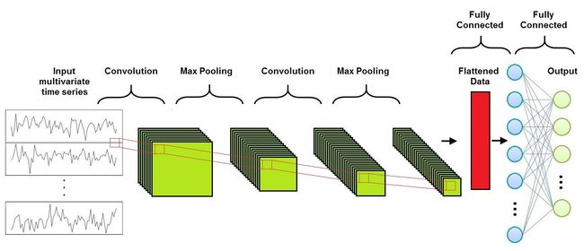
As we can see in this Figure, a Convolutional Neural Network is composed of three different layers:
如图所示,卷积神经网络由三个不同的层组成:
- Convolutional Layer 卷积层
- Pooling Layer池化层
- Fully-Connected Layer全连接层
Usually several Convolutional Layers and Pooling Layers are alternated before the Fully-Connected Layer.
通常,几个卷积层和池化层在完全连接层之前是交替的。
卷积层 (Convolutional Layer)
The convolution operation gives its name to the Convolutional Neural Networks because it’s the fundamental building block of this type of network. It performs a convolution of an input series of feature maps with a filter matrix to obtain as output a different series of feature maps, with the goal to extract the high-level features.
卷积运算之所以被称为卷积神经网络,是因为它是此类网络的基本构建块。 它使用滤波器矩阵对输入的一系列特征图进行卷积,以获取不同系列的特征图作为输出,以提取高级特征。
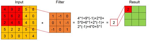
The convolution is defined by a set of filters, that are fixed size matrices. When a filter is applied to a submatrix of the input feature map with its same size, the result is given by the sum of the product of every element of the filter with the element in the same position of the submatrix (we can see this in this Figure).
卷积由一组固定大小的过滤器定义。 当将过滤器以相同的大小应用于输入要素图的子矩阵时,结果由过滤器的每个元素与子矩阵中相同位置的元素的乘积之和得出(我们可以在此图)。
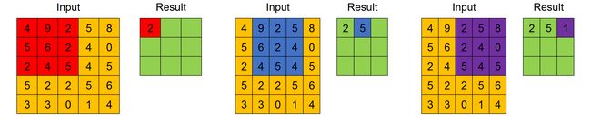
The result of the convolution between one input feature map and one filter is the ordered feature map obtained applying the filter across the width and height of the input feature map, as in this Figure.
一个输入要素图和一个过滤器之间的卷积结果就是有序特征图,该图是在输入特征图的宽度和高度上应用该过滤器而获得的,如图所示。
A Convolutional Layer executes the convolution between every filter and every input feature map, obtaining as output a series of features maps. As already underlined, the values of the filters are considered as trainable weights and then are learned during training.
卷积层执行每个过滤器和每个输入特征图之间的卷积,获得一系列特征图作为输出。 正如已经强调的那样,将过滤器的值视为可训练的权重,然后在训练过程中对其进行学习。
Two important parameters that must be chosen for the Convolutional Layer are stride and padding.
卷积层必须选择的两个重要参数是stride和padding 。
大步走 (Stride)
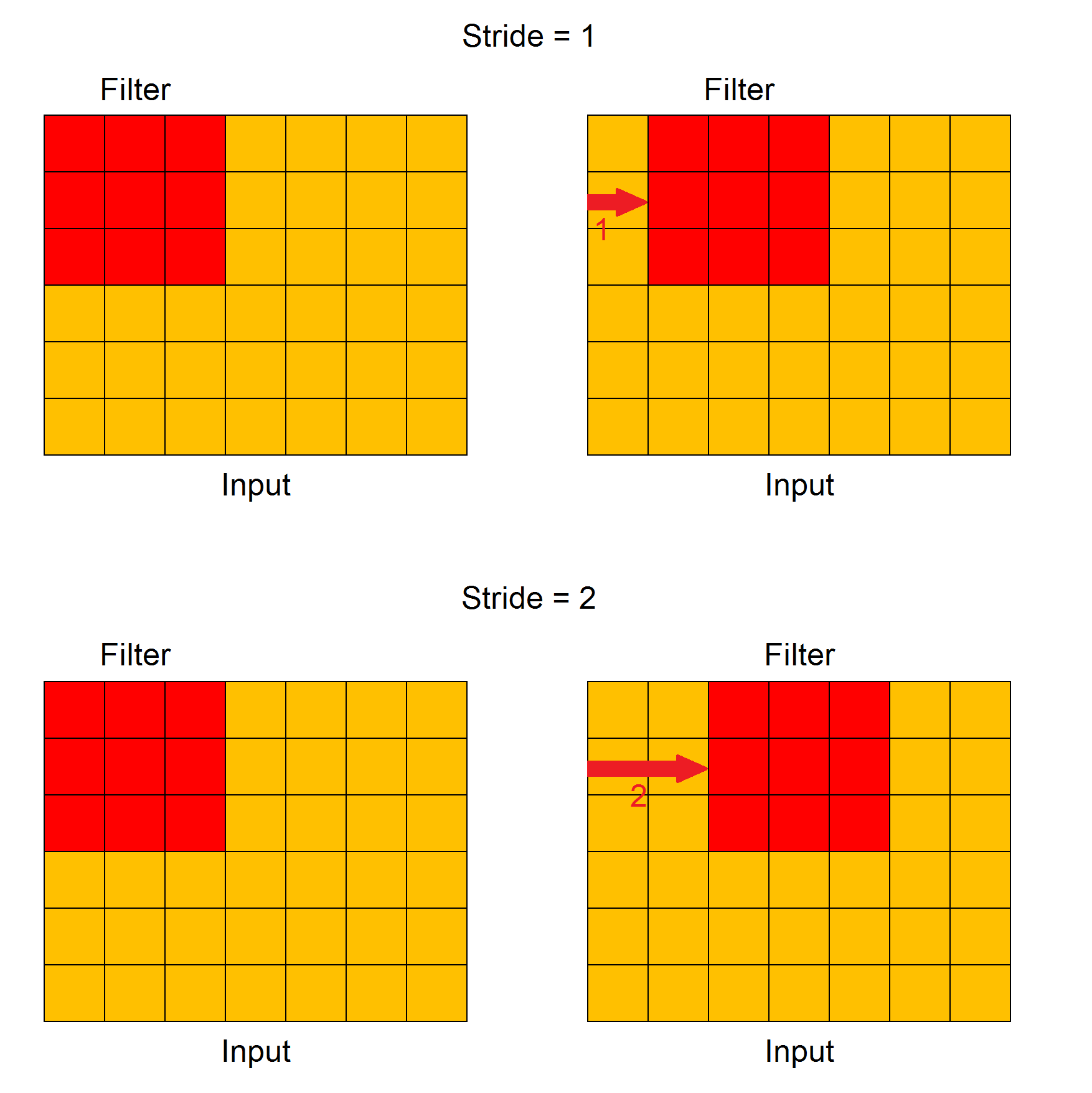
Stride controls how the filter convolves around one input feature map. In particular, the value of stride indicates how many units must be shifted at a time, how we can see in this Figure.
步幅控制过滤器如何围绕一个输入要素图进行卷积。 特别是,跨步的值表示一次必须移动多少个单位,在该图中如何显示。
填充(Padding)
Padding indicates how many extra columns and rows to add outside an input feature map, before applying a convolution filter, how we can see in this Figure. All the cells of the new columns and rows have a dummy value, usually 0.
填充指示在应用卷积过滤器之前,要在输入要素图之外添加多少额外的列和行,我们如何在此图中看到。 新列和新行的所有单元格都有一个虚拟值,通常为0。

Padding is used because when a convolution filter is applied to an input feature map, its size decreases. Then, after the application of many filter the size can become too small. Adding extra rows and columns we can preserve the original size, or make it decreasing slower.
使用填充是因为将卷积滤镜应用于输入要素图时,其大小会减小。 然后,在应用许多过滤器之后,尺寸可能变得太小。 添加额外的行和列,我们可以保留原始大小,或者使其变慢。
When the size of the feature map obtained after the application of the convolution filter is smaller than the size of the input feature map, we call this operation Valid Padding. When the output size is equal or grater of the input size, we call this operation Same Padding.
当应用卷积滤波器后获得的特征图的大小小于输入特征图的大小时,我们将此操作称为有效填充。 当输出大小等于或大于输入大小时,我们将此操作称为相同填充。
池化层 (Pooling Layer)
The purpose of pooling operation is to achieve a dimension reduction of feature maps, preserving as much information as possible. It is useful also for extracting dominant features which are rotational and positional invariant. Its input is a series of feature maps and its output is a different series of feature maps, with lower dimension.
池化操作的目的是实现特征图的降维,并保留尽可能多的信息。 这对于提取旋转和位置不变的主要特征也很有用。 它的输入是一系列特征图,其输出是不同系列的特征图,尺寸较小。
Pooling is applied to sliding windows of fixed size across the width and height of every input feature map. There are two types of pooling: Max Pooling and Average Pooling. As we can see in the Figure, for every sliding window the result of the pooling operation is its maximum value or its average value, respectively for Max Pooling or Average Pooling.
池化将应用于每个输入要素地图的宽度和高度固定大小的滑动窗口。 有两种类型的池:最大池和平均池。 从图中可以看出,对于每个滑动窗口,合并操作的结果分别是其最大值或平均值,分别是最大池化或平均池化。
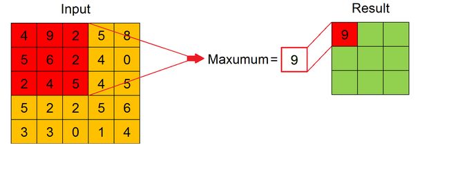
Max Pooling works also as a noise suppressant, discarding noisy activations altogether. Hence, it usually performs better than Average Pooling. Also for Pooling Layer stride and padding must be specified.
Max Pooling还可以用作噪声抑制器,完全放弃了嘈杂的激活。 因此,它通常比平均池性能更好。 同样对于池化层,必须指定步幅和填充。
The advantage of pooling operation is down-sampling the convolutional output bands, thus reducing variability in the hidden activations.
合并操作的优点是对卷积输出带进行下采样,从而减少了隐藏激活的可变性。
全连接层 (Fully-Connected Layer)
The goal of the Fully-Connected Layer is to learn non-linear combinations of the high-level features represented by the output of the Convolutional Layer and the Pooling Layer. Usually the Fully Connected Layer is implemented with a Multi Layer Perceptron.
全连接层的目标是学习由卷积层和池化层的输出表示的高级特征的非线性组合。 通常,完全连接层是使用多层感知器实现的。
After several convolution and pooling operations, the original time series is represented by a series of feature maps. All these feature maps are flattened into a column vector, that is the final representation of the original input multivariate time series. The flattened column is connected to the Multi-Layer Perceptron, whose output has a number of neurons equal to the number of possible classes of time series.
经过几次卷积和池化操作后,原始时间序列由一系列特征图表示。 所有这些特征图均被平整为列向量,即原始输入多元时间序列的最终表示。 扁平列连接到多层感知器,该感知器的输出所具有的神经元数量等于时间序列的可能类别的数量。
Backpropagation is applied to every iteration of training. Over a series of epochs, the model is able to distinguish the input time series thanks to their dominant high-level features and to classify them.
反向传播应用于训练的每个迭代。 在一系列时期中,该模型能够凭借其主要的高级功能来区分输入时间序列并对其进行分类。
超参数 (Hyperparameters)
For Convolutional Neural Networks neural network there are numerous hyperparameters to specify. The most important are the following:
对于卷积神经网络神经网络,有许多要指定的超参数。 最重要的是以下内容:
Number of convolution filters - Obviously too few filters cannot extract enough features to achieve classification. However, more filters are helpless when the filters are already enough to represent the relevant features, and make the training more computationally expensive.
卷积过滤器的数量-显然,太少的过滤器无法提取足够的特征来实现分类。 但是,当过滤器已经足以表示相关特征时,更多的过滤器将变得无能为力,并使训练在计算上更加昂贵。
Convolution filter size and initial values - Smaller filters collect as much local information as possible, bigger filters represent more global, high level and representative information. The filters are usually initialized with random values.
卷积过滤器的大小和初始值-较小的过滤器收集尽可能多的本地信息,较大的过滤器代表更多的全局,高级和代表性信息。 过滤器通常使用随机值初始化。
Pooling method and size - As already mentioned, there are two types of pooling: Max Pooling and Average Pooling, and Max Pooling usually performs better since it works also as noise suppressant. Also the pooling size is an important parameter to be optimized, since if the the pooling size increases, the dimension reduction is greater, but more informations are lost.
池化方法和大小-如前所述,池化有两种类型:“最大池化”和“平均池化”,“最大池化”通常表现更好,因为它也可以作为噪声抑制器。 而且,合并大小是要优化的重要参数,因为如果合并大小增加,则尺寸减小更大,但是会丢失更多信息。
Weight initialization - The weights are usually initialized with small random numbers to prevent dead neurons, but not too small to avoid zero gradient. Uniform distribution usually works well.
权重初始化-权重通常使用较小的随机数进行初始化,以防止神经元死亡,但也不能太小,以免出现零梯度。 均匀分布通常效果很好。
Activation function - Activation function introduces non-linearity to the model. Rectifier, sigmoid or hyperbolic tangent are usually chosen.
激活函数-激活函数将非线性引入模型。 通常选择整流器,S形或双曲线正切。
Number of epochs - Number of epochs is the the number of times the entire training set pass through the model. This number should be increased until there is a small gap between the test error and the training error, if the computational performances allow it.
时期数-时期数是整个训练集通过模型的次数。 如果计算性能允许,则应增加该数量,直到测试误差和训练误差之间存在很小的差距为止。
实作 (Implementation)
Building a Convolutional Neural Network is very easy using Keras. Keras is a simple-to-use but powerful deep learning library for Python. To build a Convolutional Neural Network in Keras are sufficient few steps:
使用Keras,构建卷积神经网络非常容易。 Keras是一个简单易用但功能强大的Python深度学习库。 要在Keras中建立卷积神经网络,只需几个步骤:
- First of all, declare a Sequential class; every Keras model is either built using the Sequential class, which represents a linear stack of layers, or the Model class, which is more flexible. Since a CNN is a linear stack of layers, we can use the simpler Sequential class; 首先,声明一个顺序类; 每个Keras模型要么使用表示线性层堆栈的Sequential类构建,要么使用更灵活的Model类构建。 由于CNN是线性的图层堆栈,因此我们可以使用更简单的Sequential类;
- Add the desired Convolutional, MaxPooling and Dense Keras Layers in the Sequential class; 在Sequential类中添加所需的卷积,MaxPooling和Dense Keras层;
- Specify number of filters and filter size for Convolutional Layer; 指定卷积层的过滤器数量和过滤器大小;
- Specify pooling size for Pooling Layer. 为池化层指定池化大小。
To compile the model, Keras needs more informations, that are:
要编译模型,Keras需要更多信息,这些信息是:
input shape (once that the input shape is specified, Keras automatically infers theshapes of inputs for later layers);
输入形状(一旦指定了输入形状,Keras会自动推断出输入形状,供以后的图层使用);
optimizer (for example Stochastic gradient descent or Adagrad);
优化器(例如随机梯度下降或Adagrad);
loss function (for example mean squared error or mean absolute percentage error);
损失函数(例如均方误差或平均绝对百分比误差);
list of metrics (for example accuracy).
指标列表(例如准确性)。
Training a model in Keras literally consists only of calling function fit() specifying the needed parameters, that are:
从Keras训练模型实际上仅包括调用函数fit()来指定所需的参数,这些参数是:
training data (input data and labels),
训练数据(输入数据和标签),
number of epochs (iterations over the entire dataset) to train for,
要训练的时期数(整个数据集的迭代次数),
validation data, which is used during training to periodically measure the network’s performance against data it hasn’t seen before.
验证数据,在训练期间用于根据以前从未见过的数据定期测量网络的性能。
Using the trained model to make predictions is easy: we pass an array of inputs to the function predict() and it returns an array of outputs.
使用训练有素的模型进行预测很容易:我们将输入数组传递给函数predict() ,并返回输出数组。
开始时间 (Inception Time)
Recently was introduced a deep Convolutional Neural Network called Inception Time. This kind of network shows high accuracy and very good scalability.
最近,引入了一种称为“开始时间”的深层卷积神经网络。 这种网络显示出很高的准确性和很好的可扩展性。
初始网络架构 (Inception Network Architecture)
The Architecture of an Inception Network is similar to the one of a Convolutional Neural Network, with the difference that Convolutional Layers and Pooling Layers are replaced with Inception Modules.
Inception网络的体系结构类似于卷积神经网络的体系结构,不同之处在于,卷积层和池化层被Inception模块替代。
As shown in this Figure, the Inception Network consists of a series of Inception Modules followed by a Global Average Pooling Layer and a Fully Conencted Layer (usually a Multi Layer Perceptron). Moreover, a residual connections is added at every third inception module. Each residual block’s input is transferred via a shortcut linear connection to be added to the next block’s input, thus mitigating the vanishing gradient problem by allowing a direct flow of the gradient.
如该图所示,Inception网络由一系列Inception模块组成,其后是全局平均池层和完全浓缩层(通常是多层感知器)。 此外,在每个第三个启动模块处添加一个剩余连接。 每个残差块的输入都通过快捷线性连接进行传输,以添加到下一个块的输入,从而通过允许梯度的直接流动来减轻消失的梯度问题。
初始模块 (Inception Module)
The major building block of an Inception Network is the Inception Module, shown in this Figure.
Inception网络的主要构建模块是Inception模块,如图所示。
It consists of 4 Layers:
它包括4层:
- The first layer is a bottleneck layer, that reduces the dimensionality of the inputs. This reduces also the computational cost and the number of parameters, speeding up training and improving generalization. 第一层是瓶颈层,它降低了输入的维数。 这也降低了计算成本和参数数量,加快了训练速度并提高了泛化能力。
- The second major component of the Inception Module is a set of parallel Convolutional Layers of different size acting on the same input feature map. For example in the Figure there are three different convolutions with filter size 10, 20, and 40. 盗取模块的第二个主要组件是一组作用在同一输入要素图上的大小不同的并行卷积层。 例如,在图中,存在三个不同的卷积,滤波器大小分别为10、20和40。
- The third layer is a MaxPooling, that introduces the ability of having a model that is invariant to small perturbations. 第三层是MaxPooling,它引入了具有对小扰动不变的模型的功能。
- The fourth and last layer is a Depth Concatenation Layer, where the output of each independent parallel convolution and of the MaxPooling is concatenated to form the output multivariate time series of the current Inception Module. 第四层也是最后一层是深度连接层,其中每个独立并行卷积和MaxPooling的输出被连接起来以形成当前Inception模块的输出多元时间序列。
By stacking multiple Inception Modules and training the filters’ values via backpropagation, the network is able to extract latent hierarchical features of multiple resolutions thanks to the use of filters with different sizes. This is the big advantage of the Inception Module since it allows the internal layers to pick and choose which filter size is relevant to learn the required information. This is very helpful to identify a high-level feature that can have different sizes on different input feature maps.
通过堆叠多个Inception模块并通过反向传播训练滤波器的值,由于使用了不同尺寸的滤波器,网络能够提取出多种分辨率的潜在分层特征。 这是Inception Module的一大优势,因为它允许内部层选择与选择哪个过滤器大小有关,以学习所需的信息。 这对于识别在不同输入要素地图上可能具有不同大小的高级要素非常有帮助。
感受野 (Receptive Field)
The key parameter to understand an Inception Network is its Receptive Field. Unlike fully-connected networks, a neuron in an Inception Network depends only on a region of the input features map. This region is called Receptive Field of the neuron. Clearly, bottom-layer neurons depend on regions that are smaller than those of top-layer. Then, bottom-layer neurons are expected to capture the local structure of a time series, while the top-layer neurons are expected to identify more complex patterns.
理解Inception网络的关键参数是其接收域。 与完全连接的网络不同,Inception网络中的神经元仅取决于输入要素图的区域。 该区域称为神经元的感受野。 显然,底层神经元依赖于小于顶层神经元的区域。 然后,期望底层神经元捕获时间序列的局部结构,而期望顶层神经元识别更复杂的模式。
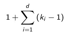
For time series data, the total Receptive field of an Inception Network is defined from this formula, that depends only on the length of the filters k_i and on depth of the network d (that is the number of Inception Modules):
对于时间序列数据,根据以下公式定义了接收网络的总接收场,该总接收场仅取决于滤波器的长度k_i和网络深度d (即接收模块的数量):
It’s very interesting to investigate how the accuracy of an Inception Network changes as the Receptive Field varies. To vary the Receptive Field we can change the filter lengths or the depth of the network.
研究接收网络随着接收场的变化如何变化的准确性非常有趣。 要改变接收场,我们可以改变滤波器的长度或网络的深度。
In most cases a longer filter is required to produce more accurate results. This is explained by the fact that longer filters are able to capture longer patterns with higher probability than shorter ones. On the contrary, increasing the Receptive Field by adding more layers doesn’t necessarily give an improvement of the network’s performance, especially for datasets with a small training set. Hence in order to improve accuracy it’s usually better to increase the filter lengths instead of adding more layers.
在大多数情况下,需要更长的过滤器才能产生更准确的结果。 这是因为较长的过滤器比较短的过滤器能够以较高的概率捕获较长的模式。 相反,通过增加更多的图层来增加“接收场”并不一定会改善网络的性能,尤其是对于训练集较小的数据集而言。 因此,为了提高精度,通常最好增加滤波器的长度,而不是增加更多的层。
起始时间架构 (Inception Time Architecture)
Many experiments have shown that a single Inception Network sometimes exhibits high variance in accuracy. This is probably because of the variability given by the random weights initialization.
许多实验表明,单个Inception Network有时会显示出较高的准确性差异。 这可能是由于随机权重初始化给出的可变性。
In order to overcome this instability, generally Inception Time is implemented as an ensemble of many Inception Networks, and every prediction has the same weight. In this way the algorithm improves his stability, and shows the already mentioned high accuracy and very good scalability.
为了克服这种不稳定性,通常将“开始时间”实现为许多“开始”网络的集合,并且每个预测都具有相同的权重。 这样,该算法提高了他的稳定性,并显示出已经提到的高精度和非常好的可伸缩性。
In particular different experiments have shown that its time complexity grows linearly with both the training set size and the time series length, and this is a very good result since many other algorithms grow quadratically with respect to the same magnitudes.
尤其是不同的实验表明,其时间复杂度随训练集大小和时间序列长度的增加而线性增加,这是一个很好的结果,因为许多其他算法相对于相同的幅度呈二次方增长。
实作 (Implementation)
A full implementation of Inception Time can be found on GitHub (https://github.com/hfawaz/InceptionTime). The implementation is written in Python and uses Keras. This implementation is based on 3 main files:
可以在GitHub( https://github.com/hfawaz/InceptionTime )上找到Inception Time的完整实现。 该实现是用Python编写的,并使用Keras。 此实现基于3个主要文件:
file main.py contains the necessary code to run an experiement;
文件main.py包含运行实验所需的代码;
file inception.py contains the Inception Network implementation;
文件inception.py包含Inception Network实现;
file nne.py contains the code that ensembles a set of Inception Networks.
文件nne.py包含集成了一组Inception Networks的代码。
In particular, the implementation uses the already mentioned Keras Module Class, since some layers of InceptionTime work in parallel, unlike Convolutional Neural Networks that uses Sequential Class since their layers are all in series.
特别地,该实现使用已经提到的Keras模块类,因为InceptionTime的某些层是并行工作的,与使用顺序类的卷积神经网络不同,因为它们的层都是串联的。
The code that implements the Inception Module building block is very similar to that described for Convolutional Neural Networks, since it uses Keras Layers for Convolution and MaxPooling, and hence it can be easily used or included in codes based on Keras in order to implement customized architectures.
实现Inception Module构建块的代码与针对卷积神经网络描述的代码非常相似,因为它使用Keras层进行卷积和MaxPooling,因此可以轻松地使用它或将其包含在基于Keras的代码中以实现定制的体系结构。
递归神经网络 (Recurrent Neural Networks)
Echo State Networks are a type of Recurrent Neural Networks, hence it can be useful a small introduction about them. Recurrent Neural Networks are networks of neuron-like nodes organized into successive layers, with an architecture similar to the one of standard Neural Networks. Infact, like in standard Neural Networks, neurons are divided in input layer, hidden layers and output layer. Each connection between neurons has a corresponding trainable weight.
回声状态网络是递归神经网络的一种,因此对它们进行少量介绍可能会很有用。 递归神经网络是组织成连续层的类神经元节点的网络,其架构类似于标准神经网络之一。 实际上,就像在标准神经网络中一样,神经元分为输入层,隐藏层和输出层。 神经元之间的每个连接都具有相应的可训练权重。
The difference is that in this case every neurons is assigned to a fixed timestep. The neurons in the hidden layer are also forwarded in a time dependent direction, that means that everyone of them is fully connected only with the neurons in the hidden layer with the same assigned timestep, and is connected with a one-way connection to every neuron assigned to the next timestep. The input and output neurons are connected only to the hidden layers with the same assigned timestep.
不同之处在于,在这种情况下,每个神经元都分配有固定的时间步长。 隐藏层中的神经元也以时间相关的方向转发,这意味着它们中的每个人都仅以相同的分配时间步长完全与隐藏层中的神经元连接,并且通过单向连接与每个神经元连接分配给下一个时间步。 输入和输出神经元仅以相同的分配时间步长连接到隐藏层。

Since the output of the hidden layer of one timestep is part of the input of the next timestep, the activation of the neurons is computed in time order: at any given timestep, only the neurons assigned to that timestep computes their activation.
由于一个时间步长的隐藏层的输出是下一时间步长的输入的一部分,因此神经元的激活按时间顺序进行计算:在任何给定的时间步长,只有分配给该时间步长的神经元才计算其激活。
Recurrent Neural Networks are rarely applied for Time Series Classification mainly due to three factors:
归因于以下三个因素,递归神经网络很少用于时间序列分类:
- The type of this architecture is designed mainly to predict an output for each element in the time series. 这种体系结构的类型主要用于预测时间序列中每个元素的输出。
- When trained on long time series, Recurrent Neural Networks typically suffer from the vanishing gradient problem, that means that the parameters in the hidden layers either don’t change that much or they lead to numeric instability and chaotic behavior. 在经过长时间序列训练后,递归神经网络通常会遇到梯度消失的问题,这意味着隐藏层中的参数要么变化不大,要么导致数值不稳定和混乱行为。
- The training of a Recurrent Neural Network is hard to parallelize, and is also computationally expensive. 递归神经网络的训练很难并行化,并且在计算上也很昂贵。
Echo State Networks were designed to mitigate the problems of Recurrent Neural Networks by eliminating the need to compute the gradient for the hidden layers, reducing the training time and avoiding the vanishing gradient problem. Infact many results show that Echo State Networks are really helpful to handle chaotic time series.
回声状态网络旨在通过消除对隐藏层计算梯度的需求,减少训练时间并避免消失的梯度问题来缓解递归神经网络的问题。 实际上,许多结果表明,回声状态网络确实有助于处理混沌时间序列。
回声州网络 (Echo State Networks)
As shown in the Figure, the Architecture of an Echo State Network consists of an Input Layer, a hidden Layer called Reservoir, a Dimension Reduction Layer, a Fully Connected Layer called Readout, and an Output Layer.
如图所示,回波状态网络的体系结构由输入层,称为存储层的隐藏层,降维层,称为读数的完全连接层和输出层组成。

- The Reservoir is the main building block of an Echo State Network and is organized like a sparsely connected random Recurrent Neural Network.水库是回声状态网络的主要组成部分,其组织类似于稀疏连接的随机递归神经网络。
- The Dimension Reduction algorithm is usually implemented with the Principal Component Analysis. 降维算法通常通过主成分分析实现。
- The Readout is usually implemented as Multi Layer Perceptron or a Ridge regressor. 读数通常实现为多层感知器或Ridge回归器。
The weights between the Input layer and the Reservoir and those in the Reservoir are randomly assigned and not trainable. The weights in the Readout are trainable, so that the network can learn and reproduce specific patterns.
输入层和水库之间的权重以及水库中的权重是随机分配的,不可训练。 读数中的权重是可训练的,因此网络可以学习和重现特定的模式。
水库 (Reservoir)

As already mentioned, the Reservoir is organized like a sparsely connected random Recurrent Neural Network. The Reservoir is connected to the Input Layer, and consists in a set of internal sparsely-connected neurons, and in its own output neurons. In the Reservoir there are 4 types of weights:
如前所述,水库的组织方式类似于稀疏连接的随机递归神经网络。 储层连接到输入层,由一组内部稀疏连接的神经元及其自身的输出神经元组成。 在水库中,有4种重量:
input weights between the Input Layer and the internal neurons;
输入层和内部神经元之间的输入权重;
internal weights, that connect the internal neurons to each other;
内部权重,将内部神经元彼此连接;
output weights between the internal neurons and the output;
内部神经元和输出之间的输出权重;
backpropagation weights, that connect back the output to the internal neurons. All these weights are randomly initialized, are equal for every time step and are not trainable.
反向传播权重,将输出连接回内部神经元。 所有这些权重都是随机初始化的,每个时间步均相等且不可训练。
Like in RNNs, the output of the Reservoir is computed separately for every time step since the output of a time step is part of the input of the next time step. At every time step, the activation of every internal and output neuron is computed, and the output for the current timestep is obtained.
像在RNN中一样,由于时间步长的输出是下一个时间步长的输入的一部分,因此每个时间步长都会分别计算水库的输出。 在每个时间步长,计算每个内部神经元和输出神经元的激活,并获得当前时间步长的输出。
The big advantage of ESNs is that the Reservoir creates a recurrent non linear embedding of the input into a higher dimension representation, but since only the weights in the Readout are trainable, the training computation time remains low.
ESN的一大优势在于,水库可以将输入重复非线性地嵌入到较高维度的表示中,但是由于只有读数中的权重是可训练的,因此训练计算时间仍然很短。
降维 (Dimension Reduction)
Many experiments show that choosing the correct dimension reduction it’s possible to reduce the execution time without lowering the accuracy. Moreover dimensional reduction provides a regularization that improves the overall generalization capability and robustness of the models.
许多实验表明,选择正确的尺寸缩减可以在不降低精度的情况下减少执行时间。 此外,降维提供了一种正则化功能,可提高模型的整体归纳能力和鲁棒性。
In most cases the training time increases almost linearly with the subspace dimension, while the accuracy quickly increases as long as the subspace dimension is below a certain threshold, then after this threshold it slows down strongly and remains almost constant. Hence this threshold is the best choice for the subspace dimension since with a higher value we would have a longer execution time without relevant improvements in the accuracy.
在大多数情况下,训练时间几乎随子空间维数线性增加,而只要子空间维数低于某个阈值,则精度就会Swift提高,然后在此阈值后,它会大大降低并保持几乎恒定。 因此,此阈值是子空间维数的最佳选择,因为如果使用更高的值,则执行时间会更长,而不会在准确性方面进行相应的改进。
实作 (Implementation)
A full implementation in Python of Echo State Networks is available on GitHub (https://github.com/FilippoMB/Reservoir-Computing-framework-for-multivariate-time-series-classification). The code uses the libraries Scikit-learn and SciPy. The main class RC_classifier contained in the file modules . py permits to build, train and test a Reservoir Computing classifier, that is the family of algorithms to which the Echo State Networks belong.
GitHub( https://github.com/FilippoMB/Reservoir-Computing-framework-for-multivariate-time-series-classification )上提供了Echo State Networks的Python完整实现。 该代码使用Scikit-learn和SciPy库。 主要模块RC_classifier包含在文件模块中。 py允许构建,训练和测试Reservoir Computing分类器,这是Echo状态网络所属的算法系列。
The hyperparameters requested for the Reservoir must be optimized in order to obtain the desired accuracy and the desired performance for the execution time; the most important are:
必须优化为水库请求的超参数,以便在执行时间内获得所需的精度和所需的性能。 最重要的是:
- the number of neurons in the Reservoir; 水库中神经元的数量;
- the percentage of nonzero connection weights (usually less then 10%); 非零连接权重的百分比(通常小于10%);
- the largest eigenvalue of the reservoir matrix of connection weights. 连接权重的储层矩阵的最大特征值。
The most important hyperparameters in other layers are:
其他层中最重要的超参数是:
- the algorithm for Dimensional Reduction Layer (that can be None or tensorial PCA for multivariate time series data); 降维层算法(对于多元时间序列数据,可以为None或张量PCA);
- the subspace dimension after the Dimension Reduction Layer; 降维层之后的子空间尺寸;
- the type of Readout used for classification (Multi Layer Perceptron, Ridge regression, or SVM); 用于分类的读数类型(多层感知器,岭回归或SVM);
- the number of epochs, that is the number iterations during the optimization. 纪元数,即优化过程中的迭代次数。
The structure of the code that implements training and uses of the model is very similar to that described for Convolutional Neural Networks.
实现模型训练和使用的代码结构与卷积神经网络非常相似。
结论 (Conclusions)
Convolutional Neural Networks are the most popular Deep Learning technique for Time Series Classifications, since they are able to successfully capture the spatial and temporal patterns through the use of trainable filters, assigning importance to these patterns using trainable weights.
卷积神经网络是用于时间序列分类的最流行的深度学习技术,因为它们能够通过使用可训练的滤波器成功捕获空间和时间模式,并使用可训练的权重将这些模式赋予重要性。
The main difficulty in using CNNs is that they are very dependent on the size and quality of the training data. In particular, the length of the time series can slow down training, and results can be not accurate as expected with chaotic input time series or with input time series in which the same relevant feature can have different sizes. To solve this problems, many new algorithms were recently elaborated, and among these InceptionTime and Echo State Networks perform better than the others.
使用CNN的主要困难在于,它们非常依赖于训练数据的大小和质量。 特别是,时间序列的长度可能会减慢训练速度,并且结果可能无法如混乱的输入时间序列或具有相同相关特征可以具有不同大小的输入时间序列所预期的那样准确。 为了解决这个问题,最近开发了许多新算法,其中InceptionTime和Echo State Networks的性能要优于其他算法。
InceptionTime is derived from Convolution Neural Networks and speeds up the training process using an efficient dimension reduction in the most important building block, the Inception Module. Moreover it performs really well in handling input time series in which the same relevant feature can have different sizes.
InceptionTime是从卷积神经网络派生而来的,它通过在最重要的构建模块Inception模块中有效地减少尺寸来加快训练过程。 此外,它在处理输入时间序列(其中相同的相关要素可以具有不同的大小)方面表现非常好。
Echo State Networks are based on Recurrent Neural Networks, and speed up the training process because they are very sparsely connected, with most of their weights fixed a priori to randomly chosen values. Thanks to this, they demonstrate remarkable performances after very fast training. Moreover they are really helpful to handle chaotic time series.
回声状态网络基于递归神经网络,由于它们之间的连接非常稀疏,并且它们的大多数权重先验地固定为随机选择的值,因此可以加快训练过程。 因此,他们在经过非常快速的培训后表现出了非凡的表现。 此外,它们对于处理混沌时间序列确实很有帮助。
Hence, in conclusion, high accuracy and high scalability make these new architectures the perfect candidate for product development.
因此,总而言之,高精度和高可扩展性使这些新架构成为产品开发的理想之选。
翻译自: https://towardsdatascience.com/time-series-classification-with-deep-learning-d238f0147d6f