图像识别和目标检测系列（Part 1）基于传统计算机视觉技术的图像识别简介

This is a multipart post on image recognition and object detection.
欢迎来到「图像识别和目标检测」系列博文，这是第一篇。

In this part, we will briefly explain image recognition using traditional computer vision techniques. I refer to techniques that are not Deep Learning based as traditional computer vision techniques because they are being quickly replaced by Deep Learning based techniques. That said, traditional computer vision approaches still power many applications. Many of these algorithms are also available in computer vision libraries like OpenCV and work very well out of the box.
在本文中，我们将简要讲述利用传统计算机视觉技术实现图像识别。我将不基于深度学习的技术称为传统的计算机视觉技术，因为它们正迅速被基于深度学习的技术所取代。也就是说，传统的计算机视觉方法仍可为许多应用程序提供支持。 其中许多算法也可以在OpenCV之类的计算机视觉库中使用，并且开箱即用。

This series will follow the following rough outline.

1. Image recognition using traditional Computer Vision techniques :
2. Part 1 Histogram of Oriented Gradients : Part 2
3. Example code for image recognition : Part 3
4. Training a better eye detector: Part 4a
5. Object detection using traditional Computer Vision techniques : Part4b
6. How to train and test your own OpenCV object detector : Part 5
7. Image recognition using Deep Learning : Part 6
   • Introduction to Neural Networks
   • Understanding Feedforward Neural Networks Image
   • Recognition using Convolutional Neural Networks
8. Object detection using Deep Learning : Part 7

图像识别和目标检测简史

Our story begins in 2001; the year an efficient algorithm for face detection was invented by Paul Viola and Michael Jones. Their demo that showed faces being detected in real time on a webcam feed was the most stunning demonstration of computer vision and its potential at the time. Soon, it was implemented in OpenCV and face detection became synonymous with Viola and Jones algorithm.
我们的故事始于2001年； Paul Viola和Michael Jones发明了一种效率很高的人脸检测算法。 他们的演示显示了在网络摄像头上实时检测到的面部，这是当时计算机视觉及其潜力的最令人震惊的演示。 很快，它在OpenCV中实现，面部检测成为Viola和Jones算法的代名词。

Every few years a new idea comes along that forces people to pause and take note. In object detection, that idea came in 2005 with a paper by Navneet Dalal and Bill Triggs. Their feature descriptor, Histograms of Oriented Gradients (HOG), significantly outperformed existing algorithms in pedestrian detection.
每隔几年就会出现一个新想法，迫使人们停下来并记笔记。 在目标检测领域中，有个想法是在2005年由Navneet Dalal和Bill Triggs发表的论文提出的。 它们的特征描述子“方向梯度直方图（HOG）”在行人检测中明显优于现有算法。

Every decade or so a new idea comes along that is so effective and powerful that you abandon everything that came before it and wholeheartedly embrace it. Deep Learning is that idea of this decade. Deep Learning algorithms had been around for a long time, but they became mainstream in computer vision with its resounding success at the ImageNet Large Scale Visual Recognition Challenge (ILSVRC) of 2012. In that competition, an algorithm based on Deep Learning by Alex Krizhevsky, Ilya Sutskever, and Geoffrey Hinton shook the computer vision world with an astounding 85% accuracy — 11% better than the algorithm that won the second place! In ILSVRC 2012, this was the only Deep Learning based entry. In 2013, all winning entries were based on Deep Learning and in 2015 multiple Convolutional Neural Network (CNN) based algorithms surpassed the human recognition rate of 95%.
每隔十年左右，就会出现一个如此有效和有力的新想法，以至于您放弃之前的一切，全心全意地接受它。 深度学习就是这个十年的想法。 深度学习算法已经存在了很长时间，但是由于在2012年ImageNet大规模视觉识别挑战赛（ILSVRC）上取得了巨大成功，它们已成为计算机视觉的主流。在该竞赛中，基于Alex Krizhevsky、Ilya Sutskever和Geoffrey Hinton的“深度学习”算法， 以惊人的85％的准确性震撼了计算机视觉世界，比赢得第二名的算法高11％！ 在ILSVRC 2012中，这是唯一基于深度学习的条目。 2013年，所有获奖作品均基于深度学习，2015年，基于多个卷积神经网络（CNN）的算法的人类识别率超过了95％。

With such huge success in image recognition, Deep Learning based object detection was inevitable. Techniques like Faster R-CNN produce jaw-dropping results over multiple object classes. We will learn about these in later posts, but for now keep in mind that if you have not looked at Deep Learning based image recognition and object detection algorithms for your applications, you may be missing out on a huge opportunity to get better results.
凭借在图像识别方面的巨大成功，基于深度学习的目标检测是不可避免的。 诸如Faster R-CNN之类的技术会在多目标分类上产生令人结舌的结果。 我们将在以后的文章中学习这些内容，但是现在请记住，如果您还没有研究针对应用程序的使用基于深度学习的图像识别和目标检测算法，那么您可能会错失了获得更好结果的巨大机会。

有了这一概述，我们准备返回本文的主要目标——理解使用传统计算机视觉技术的图像识别。

图像识别（又称图像分类）

An image recognition algorithm ( a.k.a an image classifier ) takes an image ( or a patch of an image ) as input and outputs what the image contains. In other words, the output is a class label ( e.g. “cat”, “dog”, “table” etc. ). How does an image recognition algorithm know the contents of an image ? Well, you have to train the algorithm to learn the differences between different classes. If you want to find cats in images, you need to train an image recognition algorithm with thousands of images of cats and thousands of images of backgrounds that do not contain cats. Needless to say, this algorithm can only understand objects / classes it has learned.
图像识别算法（也称为图像分类器）将图像（或图像的一部分）作为输入并输出图像包含的内容。 换句话说，输出是类别标签（例如“猫”，“狗”，“桌子”等）。 图像识别算法如何知道图像的内容？ 好吧，您必须通过学习不同类之间的差异去训练算法。 如果要在图像中找到猫，则需要通过包含成千上万的猫图像和成千上万的不包含猫的背景图像，训练一种图像识别算法。不用说，该算法只能理解它已经学到的对象/类。

To simplify things, in this post we will focus only on two-class (binary) classifiers. You may think that this is a very limiting assumption, but keep in mind that many popular object detectors ( e.g. face detector and pedestrian detector ) have a binary classifier under the hood. E.g. inside a face detector is an image classifier that says whether a patch of an image is a face or background.
为简化起见，在本文中，我们将仅着眼于两类（二分类）分类器。 您可能会认为这个假设局限性很大，但请记住，许多流行的物体检测器（例如面部检测器和行人检测器）在内部都有一个二进制分类器。 例如，人脸检测器内部是一个图像分类器，用于区分图像的这块是人脸还是背景。

图像分类器的剖析

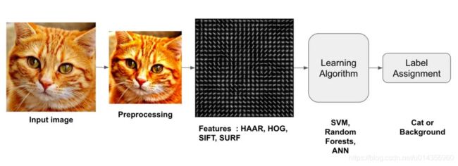
The following diagram illustrates the steps involved in a traditional image classifier.
下图说明了传统图像分类器分类的步骤。

Interestingly, many traditional computer vision image classification algorithms follow this pipeline, while Deep Learning based algorithms bypass the feature extraction step completely. Let us look at these steps in more details.
有趣的是，许多传统的计算机视觉图像分类算法都遵循这一流程，而基于深度学习的算法则完全绕过了特征提取步骤。 让我们更详细地了解这些步骤。

Step 1 : Preprocessing 预处理

Often an input image is pre-processed to normalize contrast and brightness effects. A very common preprocessing step is to subtract the mean of image intensities and divide by the standard deviation. Sometimes, gamma correction produces slightly better results. While dealing with color images, a color space transformation ( e.g. RGB to LAB color space ) may help get better results.
通常，对输入图像进行预处理的目的是，对比度和亮度进行归一化。一个非常常见的预处理步骤是：从原图像减去图像强度的平均值，然后除以标准偏差。有时，伽马校正会产生更好的结果。在处理彩色图像时，颜色空间转换（例如RGB到LAB颜色空间）可能有助于获得更好的结果。

Notice that I am not prescribing what pre-processing steps are good. The reason is that nobody knows in advance which of these preprocessing steps will produce good results. You try a few different ones and some might give slightly better results. Here is a paragraph from Dalal and Triggs
请注意，我没有规定哪些预处理步骤是好的。原因是没有人事先知道这些预处理步骤中的哪些会产生良好的结果。您尝试几种不同的方法，有些可能会产生更好的结果。这是Dalal和Triggs的一段话：

“We evaluated several input pixel representations including grayscale, RGB and LAB colour spaces optionally with power law (gamma) equalization. These normalizations have only a modest effect on performance, perhaps because the subsequent descriptor normalization achieves similar results. We do use colour information when available. RGB and LAB colour spaces give comparable results, but restricting to grayscale reduces performance by 1.5% at 10−4 FPPW. Square root gamma compression of each colour channel improves performance at low FPPW (by 1% at 10−4 FPPW) but log compression is too strong and worsens it by 2% at 10−4 FPPW.”
“我们评估了几种不同图像的表示方法，包括灰度图像，RGB图像和LAB颜色空间的图像，并在某些图像上进行了幂律（gamma）均衡。这些归一化对性能的影响不大，可能是因为后续的描述符归一化获得了相似的结果。当有彩色图片时，我们实验采用彩色图片。 RGB和LAB颜色空间产生的结果相似，但在10−4 FPPW时，限制灰度将会使性能降低1.5％。对每个色彩通道采用平方根伽玛压缩，当FPPW较低时，可提高性能（在10−4 FPPW时提高1％），但在10−4 FPPW时，对数压缩太强，会使性能降低2％。”
【FPPW基本含义：给定一定数目N的负样本图像，分类器将负样本判定为“正”的次数FP，其比率FP/N即为FPPW。意义与ROC中的假阳率相同。FPPW中，一张图就是一个样本。】

As you can see, they did not know in advance what pre-processing to use. They made reasonable guesses and used trial and error.
如您所见，他们事先不知道要使用什么预处理。他们做出了合理的猜测，并使用了反复试验。

As part of pre-processing, an input image or patch of an image is also cropped and resized to a fixed size. This is essential because the next step, feature extraction, is performed on a fixed sized image.
作为预处理的一部分，还会将图像或部分图像裁剪并将其调整为固定大小。这是必不可少的，因为下一步是对固定大小的图像执行特征提取。

Step 2 : Feature Extraction 特征提取

The input image has too much extra information that is not necessary for classification. Therefore, the first step in image classification is to simplify the image by extracting the important information contained in the image and leaving out the rest. For example, if you want to find shirt and coat buttons in images, you will notice a significant variation in RGB pixel values. However, by running an edge detector on an image we can simplify the image. You can still easily discern the circular shape of the buttons in these edge images and so we can conclude that edge detection retains the essential information while throwing away non-essential information. The step is called feature extraction. In traditional computer vision approaches designing these features are crucial to the performance of the algorithm. Turns out we can do much better than simple edge detection and find features that are much more reliable. In our example of shirt and coat buttons, a good feature detector will not only capture the circular shape of the buttons but also information about how buttons are different from other circular objects like car tires.
输入图像包含过多的与分类无关的信息。因此，图像分类的第一步是简化图像。它是通过提取图像中包含的重要信息并忽略其余信息来实现的。例如，如果要在图像中找到衬衫和外套纽扣，您会注意RGB像素值有很大变化的地方。但是，通过在图像上运行边缘检测器，我们可以简化图像。您仍然可以轻松地辨别这些边缘图像中按钮的圆形形状，因此我们可以得出结论，边缘检测保留了基本信息而丢弃了不必要的信息。该步骤称为特征提取。在传统的计算机视觉方法中，设计这些功能对于算法的性能至关重要。事实证明，与简单的边缘检测相比，我们可以做的更好，并且找到更可靠的功能。在我们的衬衫纽扣和外套纽扣示例中，好的功能检测器不仅会捕获纽扣的圆形形状，还会获取有关纽扣与其他圆形物体（例如汽车轮胎）的区别。

Some well-known features used in computer vision are Haar-like features introduced by Viola and Jones, Histogram of Oriented Gradients ( HOG ), Scale-Invariant Feature Transform ( SIFT ), Speeded Up Robust Feature ( SURF ) etc.
计算机视觉中使用的一些著名特征包括Viola和Jones引入的类Haar特征，方向梯度直方图（HOG），尺度不变特征变换（SIFT），**加速鲁棒特征（SURF）**等。

As a concrete example, let us look at feature extraction using Histogram of Oriented Gradients ( HOG ).
作为一个具体的例子，让我们看一下使用方向梯度直方图（HOG）进行特征提取。

Histogram of Oriented Gradients ( HOG )

A feature extraction algorithm converts an image of fixed size to a feature vector of fixed size. In the case of pedestrian detection, the HOG feature descriptor is calculated for a 64×128 patch of an image and it returns a vector of size 3780. Notice that the original dimension of this image patch was 64 × 128 × 3 = 24,576 which is reduced to 3780 by the HOG descriptor.
特征提取算法将固定大小的图像转换为固定大小的特征向量。在行人检测的情况下，将为分辨率为64×128的子图计算HOG特征描述符，并返回大小为3780的向量。请注意，此图像色块的原始尺寸为$64\times 128\times 3=24,576$，即由HOG描述符减少到3780。

HOG is based on the idea that local object appearance can be effectively described by the distribution ( histogram ) of edge directions ( oriented gradients ). The steps for calculating the HOG descriptor for a 64×128 image are listed below.
HOG基于这样的思想，即可以通过边缘方向（方向梯度）的分布（直方图）有效地描述局部对象的外观。下面列出了计算分辨率为64×128图像的HOG描述符的步骤。

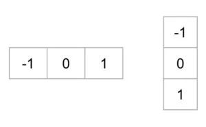
1. Gradient calculation : Calculate the x and the y gradient images, $g_x$ and $g_y$, from the original image. This can be done by filtering the original image with the following kernels.
   梯度计算：从原始图像上计算x和y梯度图像，$g_x$和$g_y$。这可以通过使用以下kernel过滤原始图像来完成。
   
   Using the gradient images $g_x$ and $g_y$, we can calculate the magnitude and orientation of the gradient using the following equations.
   使用梯度图像$g_x$和$g_y$，我们可以使用以下公式计算梯度的大小和方向。
   $$\begin{gathered} g=\sqrt{g_x^2+g_y^2} \\ \theta =\arctan \frac{g_y}{g_x} \end{gathered}$$
   The calcuated gradients are “unsigned” and therefore \theta is in the range 0 to 180 degrees.
   计算得出的梯度是“无符号的”，因此$\theta$在0到180度的范围内。

2. Cells : Divide the image into 8×8 cells.
   单元格：将图像划分，使8×8为一单元格。

3. Calculate histogram of gradients in these 8×8 cells : At each pixel in an 8×8 cell we know the gradient ( magnitude and direction ), and therefore we have 64 magnitudes and 64 directions — i.e. 128 numbers. Histogram of these gradients will provide a more useful and compact representation. We will next convert these 128 numbers into a 9-bin histogram ( i.e. 9 numbers ). The bins of the histogram correspond to gradients directions 0, 20, 40 … 160 degrees. Every pixel votes for either one or two bins in the histogram. If the direction of the gradient at a pixel is exactly 0, 20, 40 … or 160 degrees, a vote equal to the magnitude of the gradient is cast by the pixel into the bin. A pixel where the direction of the gradient is not exactly 0, 20, 40 … 160 degrees splits its vote among the two nearest bins based on the distance from the bin. E.g. A pixel where the magnitude of the gradient is 2 and the angle is 20 degrees will vote for the second bin with value 2. On the other hand, a pixel with gradient 2 and angle 30 will vote 1 for both the second bin ( corresponding to angle 20 ) and the third bin ( corresponding to angle 40 ).
   计算这些8×8子图中的梯度直方图：在8×8子图中的每个像素处，我们都知道它的梯度（大小和方向），因此，我们有64个梯度大小和64个梯度方向（即128个数字）。梯度直方图是对这些信息更加有用和紧凑的表示方法。接下来，我们将把这128个数字转换为9-bin直方图（即9个数字）。直方图的每个bin对应于梯度方向0、20、40、60、80、100、120、140、160度。每个像素点将对应于直方图中的一个或两个bin。如果某个像素处的渐变方向正好是0、20、40…或160度，则该像素将等于该渐变大小的投票投到bin中。渐变方向不完全为0、20、40…160度的像素会根据距bin的距离在两个最近的像素仓中分配其投票。例如，梯度大小为2且方向为20°的像素点将投票给角度为20的bin，票数为2。另一方面，梯度大小为2且方向为30的像素，将投票给第二个bin（对应于角度20）和第三个bin（对应于角度40），票数各为1。

4. Block normalization : The histogram calculated in the previous step is not very robust to lighting changes. Multiplying image intensities by a constant factor scales the histogram bin values as well. To counter these effects we can normalize the histogram — i.e. think of the histogram as a vector of 9 elements and divide each element by the magnitude of this vector. In the original HOG paper, this normalization is not done over the 8×8 cell that produced the histogram, but over 16×16 blocks. The idea is the same, but now instead of a 9 element vector you have a 36 element vector.
   块归一化：上一步中计算出的直方图对照明变化的鲁棒性不是很强。将图像强度乘以恒定因子（光照带来的影响，译者注）也会缩放直方图中bin的值。为了抵消这些影响，我们可以将直方图归一化-例如，将直方图视为9个元素的向量，然后将每个元素除以该向量的长度。在原始HOG论文中，未对生成直方图的8×8单元格进行归一化，而是对16×16的单元块（相邻4个8×8单元格，译者注）进行了归一化。想法是一样的，这样就有了36元素的向量，而不是9元素的向量。

5. Feature Vector : In the previous steps we figured out how to calculate histogram over an 8×8 cell and then normalize it over a 16×16 block. To calcualte the final feature vector for the entire image, the 16×16 block is moved in steps of 8 ( i.e. 50% overlap with the previous block ) and the 36 numbers ( corresponding to 4 histograms in a 16×16 block ) calculated at each step are concatenated to produce the final feature vector.What is the length of the final vector ?
   特征向量：在前面的步骤中，我们弄清楚了如何在8×8单元格上计算直方图，然后在16×16块上对其进行归一化。为了计算整个图像的最终特征向量，将16×16单元块以8（即与上一个块重叠50％）的步长移动，并在每一步会计算出36个数字（对应于16×16块中的4个直方图）。将每个步骤计算出的数字连接起来以生成最终特征向量。最终向量的长度是多少？
   The input image is 64×128 pixels in size, and we are moving 8 pixels at a time. Therefore, we can make 7 steps in the horizontal direction and 15 steps in the vertical direction which adds up to 7 x 15 = 105 steps. At each step we calculated 36 numbers, which makes the length of the final vector 105 x 36 = 3780.
   输入图像的尺寸为64×128像素，我们一次移动8像素。 因此，我们可以在水平方向上进行7步，而在垂直方向上进行15步，因此总共可以达到7 x 15 = 105步。 在每一步中，我们计算了36个数字，这使得最终向量的长度为105 x 36 = 3780。

Step 3 : Learning Algorithm For Classification 分类学习算法

In the previous section, we learned how to convert an image to a feature vector. In this section, we will learn how a classification algorithm takes this feature vector as input and outputs a class label ( e.g. cat or background ).
在上一节中，我们学习了如何将图像转换为特征向量。 在本节中，我们将学习分类算法如何将特征向量作为输入并输出类标签（例如，cat或background）。

Before a classification algorithm can do its magic, we need to train it by showing thousands of examples of cats and backgrounds. Different learning algorithms learn differently, but the general principle is that learning algorithms treat feature vectors as points in higher dimensional space, and try to find planes / surfaces that partition the higher dimensional space in such a way that all examples belonging to the same class are on one side of the plane / surface.
在分类算法发挥作用之前，我们需要通过展示成千上万的猫和背景的示例来训练它。 不同的学习算法学习的方法不同，但是一般的原则是学习算法将特征向量视为高维空间中的点，并尝试查找划分高维空间的平面/曲面，使得属于同一类的所有示例都在平面/曲面的一侧。

To simplify things, let us look at one learning algorithm called Support Vector Machines ( SVM ) in some detail.
为简化起见，让我们详细了解一种称为支持向量机（SVM）的学习算法。

How does Support Vector Machine ( SVM ) Work For Image Classification? 支持向量机（SVM）如何用于图像分类？

Support Vector Machine ( SVM ) is one of the most popular supervised binary classification algorithm. Although the ideas used in SVM have been around since 1963, the current version was proposed in 1995 by Cortes and Vapnik.
支持向量机（SVM）是最流行的监督二进制分类算法之一。 尽管SVM中所使用的想法自1963年就出现了，但当前版本是由Cortes和Vapnik于1995年提出的。

In the previous step, we learned that the HOG descriptor of an image is a feature vector of length 3780. We can think of this vector as a point in a 3780-dimensional space. Visualizing higher dimensional space is impossible, so let us simplify things a bit and imagine the feature vector was just two dimensional.
在上一步中，我们学习了图像的HOG描述子是长度为3780的特征向量。我们可以将此向量视为3780维空间中的一个点。 可视化高维空间是不可能的，因此让我们稍微简化一下，并想象特征向量只是二维的。

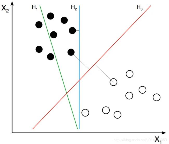
In our simplified world, we now have 2D points representing the two classes ( e.g. cats and background ). In the image above, the two classes are represented by two different kinds of dots. All black dots belong to one class and the white dots belong to the other class. During training, we provide the algorithm with many examples from the two classes. In other words, we tell the algorithm the coordinates of the 2D dots and also whether the dot is black or white.
在我们的简化世界中，我们现在有代表两个类别（例如猫和背景）的二维坐标上的点。在上图中，两个类别由两种不同类型的点表示。所有黑点属于一类，白点属于另一类。在训练期间，我们为算法提供了两类中的许多示例。换句话说，我们告诉算法二维点的坐标以及点是黑色还是白色。

Different learning algorithms figure out how to separate these two classes in different ways. Linear SVM tries to find the best line that separates the two classes. In the figure above, H1, H2, and H3 are three lines in this 2D space. H1 does not separate the two classes and is therefore not a good classifier. H2 and H3 both separate the two classes, but intuitively it feels like H3 is a better classifier than H2 because H3 appears to separate the two classes more cleanly. Why ? Because H2 is too close to some of the black and white dots. On the other hand, H3 is chosen such that it is at a maximum distance from members of the two classes.
不同的学习算法会找出如何以不同方式将这两类分开。线性SVM试图找到分隔这两个类别的最佳直线。在上图中，H1，H2和H3是此二维空间中的三条线。 H1不能将这两个类别分开，因此不是一个很好的分类器。 H2和H3都将这两个类别分开，但是直觉上感觉H3比H2更好，因为H3似乎更清晰地将这两个类别分开了。为什么呢？因为H2太靠近某些黑点和白点了。另一方面，选择H3使其距两类成员的最大距离。

Given the 2D features in the above figure, SVM will find the line H3 for you. If you get a new 2D feature vector corresponding to an image the algorithm has never seen before, you can simply test which side of the line the point lies and assign it the appropriate class label. If your feature vectors are in 3D, SVM will find the appropriate plane that maximally separates the two classes. As you may have guessed, if your feature vector is in a 3780-dimensional space, SVM will find the appropriate hyperplane.
在上述图像上的二维特征中，SVM将为您找到线H3。如果获得与算法从未见过的图像相对应的新2D特征向量，则可以简单地测试该点位于线的哪一侧，并为其分配适当的类标签。如果您的特征向量是3D模式，则SVM将找到分隔两类最大间隔的适当平面。您可能已经猜到，如果您的特征向量在3780维空间中，则SVM将找到合适的超平面。

Optimizing SVM

So far so good, but I know you have one important unanswered question. What if the features belonging to the two classes are not separable using a hyperplane ? In such cases, SVM still finds the best hyperplane by solving an optimization problem that tries to increase the distance of the hyperplane from the two classes while trying to make sure many training examples are classified properly. This tradeoff is controlled by a parameter called C. When the value of C is small, a large margin hyperplane is chosen at the expense of a greater number of misclassifications. Conversely, when C is large, a smaller margin hyperplane is chosen that tries to classify many more examples correctly.
到目前为止一切顺利，但我知道您有一个重要的未解决问题。 如果属于两类的要素无法使用超平面分离，该怎么办？ 在这种情况下，SVM仍然可以通过解决一个优化问题来找到最佳的超平面，该优化问题试图增加超平面与两个类别的距离，同时尝试确保对许多训练示例进行正确分类。 这种权衡是由称为C的参数控制的。当C的值较小时，将以较大的错误分类为代价选择较大的余量超平面。 相反，当C较大时，将选择较小的余量超平面，以尝试对更多示例进行正确分类。

Now you may be confused as to what value you should choose for C. Choose the value that performs best on a validation set that the algorithm was not trained on.
现在，您可能会对应该为C选择什么值感到困惑。选择在未经训练的算法的验证集上表现最佳的值。

Subscribe & Download Code

I hope you liked the article and it was useful. To download code (C++ and Python) and example images used in this blog, please subscribe to our newsletter. You will also receive a free Computer Vision Resource guide. In our newsletter we share OpenCV tutorials and examples written in C++/Python, and Computer Vision and Machine Learning algorithms and news.