snntorch:P2—【LIF神经元模型】手撕公式、代码实现与演示
LIF神经元模型是现阶段脉冲神经网络的搭建与训练过程中使用最多的神经元模型,既保留了HH模型中关于生物神经元的核心思想,具有一定的仿生型,也兼顾了普通人工神经元计算效率高的特点,所以本文就LIF神经元展开说明,包括了生物启发的模型建立、公式推导、离散化递归表示以用于代码实现,最后有snntorch框架中关于LIF神经元的相关代码。
L: leaky(泄露)——细胞膜内外存在电势差时,电压会逐渐降低(泄露)
I: integrate(积分)——外部向神经元注入电流时,神经元会对接收到的脉冲序列进行积分求和
F: fire(发放)——上一步的膜电压的值超过设定的阈值后,当前神经元就会发放脉冲
高中生物学告诉我们,细胞膜主要由磷脂双分子层构成,将细胞内外隔离开来,并在细胞内外形成一定的离子浓度差(静息状态下细胞膜内钾离子多,膜外钠离子多),并由此产生了一定的电势差(神经元静息状态下膜电位外正内负),磷脂双分子层就类似于一个电容的作用,当神经元接收到电流刺激时,会诱使细胞膜上一些离子通道打开,钠离子开始流入,此时的离子通道就相当于一个电阻的作用,受此启发,1907年发现这个现象的 Louis Lapicque就以一个RC电路的形式建立起了生物神经元的简化模型(准确来说应该是神经元细胞膜的简易模型),相关电路就在下图中的左上。

我们列出了一个常微分方程表示出了膜电压的计算公式(右上),并计算出了它的解析解,在输入电流为0时,膜电压会从初始电压开始,进行服从于tau = RC的指数衰减,为了便于计算机处理,我们还需要将此解进行离散化、递归处理,虽然我们人工不可能使用这种方式计算,但这种递归的形式显然适合计算机处理,以下即为这种方式的代码实现。
def plot_mem(mem, title=False):
  if title:
    plt.title(title)
  plt.plot(mem)
  plt.xlabel("Time step")
  plt.ylabel("Membrane Potential")
  plt.xlim([0, 50])
  plt.ylim([0, 1])
  plt.show()
def leaky_integrate_neuron(U, time_step=1e-3, I=0, R=5e7, C=1e-10):
  tau = R*C
  U = U + (time_step/tau)*(-U + I*R)
  return U
num_steps = 100
U = 0.9
U_trace = []  # keeps a record of U for plotting

for step in range(num_steps):
  U_trace.append(U)
  U = leaky_integrate_neuron(U)  # solve next step of U

plot_mem(U_trace, "Leaky Neuron Model")
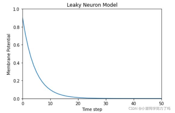
从运行结果可以看出,膜电压在输入电流为0时衰减曲线和我们解析解画出来的图像是一致的。
snntorch框架中,现在有4种 lif 的模型,通过以下调用实现。
- Lapicque’s RC model:
snntorch.Lapicque - Non-physical 1st order model:
snntorch.Leaky - Synaptic Conductance-based neuron model:
snntorch.Synaptic - Alpha neuron Model:
snntorch.Alpha
第一种 snntorch.Lapicque就是我们刚刚演示过的 RC 电路的神经元模型(起这个名字就是为了纪念 Louis Lapicque ~),来看一下它是怎么实现的(无输入电流刺激的情况下)。
import snntorch
time_step = 1e-3
R = 5
C = 1e-3
# leaky integrate and fire neuron, tau=5e-3
lif1 = snn.Lapicque(R=R, C=C, time_step=time_step)
# Initialize membrane, input, and output
mem = torch.ones(1) * 0.9  # U=0.9 at t=0
cur_in = torch.zeros(num_steps)  # I=0 for all t
spk_out = torch.zeros(1)  # initialize output spikes
# A list to store recordings of membrane potential
mem_rec = [mem]
# pass updated value of mem and cur_in[step]=0 at every time step
for step in range(num_steps):
  spk_out, mem = lif1(cur_in[step], mem)

  # Store recordings of membrane potential
  mem_rec.append(mem)

# crunch the list of tensors into one tensor
mem_rec = torch.stack(mem_rec)

plot_mem(mem_rec, "Lapicque's Neuron Model Without Stimulus")
还有一些未列出的演示,包括输入电流为阶跃信号或者脉冲信号时的膜电压的变化、神经元脉冲发放等许多功能,大家可运行如下程序查看,可以与我交流心得~
import snntorch as snn
from snntorch import spikeplot as splt
from snntorch import spikegen

import torch
import torch.nn as nn

import numpy as np
import matplotlib.pyplot as plt


def plot_mem(mem, title=False):
  if title:
    plt.title(title)
  plt.plot(mem)
  plt.xlabel("Time step")
  plt.ylabel("Membrane Potential")
  plt.xlim([0, 50])
  plt.ylim([0, 1])
  plt.show()

def plot_step_current_response(cur_in, mem_rec, vline1):
  fig, ax = plt.subplots(2, figsize=(8,6),sharex=True)

  # Plot input current
  ax[0].plot(cur_in, c="tab:orange")
  ax[0].set_ylim([0, 0.2])
  ax[0].set_ylabel("Input Current ($I_{in}$)")
  ax[0].set_title("Lapicque's Neuron Model With Step Input")

  # Plot membrane potential
  ax[1].plot(mem_rec)
  ax[1].set_ylim([0, 0.6])
  ax[1].set_ylabel("Membrane Potential ($U_{mem}$)")

  if vline1:
    ax[1].axvline(x=vline1, ymin=0, ymax=2.2, alpha = 0.25, linestyle="dashed", c="black", linewidth=2, zorder=0, clip_on=False)
  plt.xlabel("Time step")

  plt.show()


def plot_current_pulse_response(cur_in, mem_rec, title, vline1=False, vline2=False, ylim_max1=False):

  fig, ax = plt.subplots(2, figsize=(8,6),sharex=True)

  # Plot input current
  ax[0].plot(cur_in, c="tab:orange")
  if not ylim_max1:
    ax[0].set_ylim([0, 0.2])
  else:
    ax[0].set_ylim([0, ylim_max1])
  ax[0].set_ylabel("Input Current ($I_{in}$)")
  ax[0].set_title(title)

  # Plot membrane potential
  ax[1].plot(mem_rec)
  ax[1].set_ylim([0, 1])
  ax[1].set_ylabel("Membrane Potential ($U_{mem}$)")

  if vline1:
    ax[1].axvline(x=vline1, ymin=0, ymax=2.2, alpha = 0.25, linestyle="dashed", c="black", linewidth=2, zorder=0, clip_on=False)
  if vline2:
    ax[1].axvline(x=vline2, ymin=0, ymax=2.2, alpha = 0.25, linestyle="dashed", c="black", linewidth=2, zorder=0, clip_on=False)
  plt.xlabel("Time step")

  plt.show()

def compare_plots(cur1, cur2, cur3, mem1, mem2, mem3, vline1, vline2, vline3, vline4, title):
  # Generate Plots
  fig, ax = plt.subplots(2, figsize=(8,6),sharex=True)

  # Plot input current
  ax[0].plot(cur1)
  ax[0].plot(cur2)
  ax[0].plot(cur3)
  ax[0].set_ylim([0, 0.2])
  ax[0].set_ylabel("Input Current ($I_{in}$)")
  ax[0].set_title(title)

  # Plot membrane potential
  ax[1].plot(mem1)
  ax[1].plot(mem2)
  ax[1].plot(mem3)
  ax[1].set_ylim([0, 1])
  ax[1].set_ylabel("Membrane Potential ($U_{mem}$)")

  ax[1].axvline(x=vline1, ymin=0, ymax=2.2, alpha = 0.25, linestyle="dashed", c="black", linewidth=2, zorder=0, clip_on=False)
  ax[1].axvline(x=vline2, ymin=0, ymax=2.2, alpha = 0.25, linestyle="dashed", c="black", linewidth=2, zorder=0, clip_on=False)
  ax[1].axvline(x=vline3, ymin=0, ymax=2.2, alpha = 0.25, linestyle="dashed", c="black", linewidth=2, zorder=0, clip_on=False)
  ax[1].axvline(x=vline4, ymin=0, ymax=2.2, alpha = 0.25, linestyle="dashed", c="black", linewidth=2, zorder=0, clip_on=False)

  plt.xlabel("Time step")

  plt.show()

def plot_cur_mem_spk(cur, mem, spk, thr_line=False, vline=False, title=False, ylim_max2=1.25):
  # Generate Plots
  fig, ax = plt.subplots(3, figsize=(8,6), sharex=True,
                        gridspec_kw = {'height_ratios': [1, 1, 0.4]})

  # Plot input current
  ax[0].plot(cur, c="tab:orange")
  ax[0].set_ylim([0, 0.4])
  ax[0].set_xlim([0, 200])
  ax[0].set_ylabel("Input Current ($I_{in}$)")
  if title:
    ax[0].set_title(title)

  # Plot membrane potential
  ax[1].plot(mem)
  ax[1].set_ylim([0, ylim_max2])
  ax[1].set_ylabel("Membrane Potential ($U_{mem}$)")
  if thr_line:
    ax[1].axhline(y=thr_line, alpha=0.25, linestyle="dashed", c="black", linewidth=2)
  plt.xlabel("Time step")

  # Plot output spike using spikeplot
  splt.raster(spk, ax[2], s=400, c="black", marker="|")
  if vline:
    ax[2].axvline(x=vline, ymin=0, ymax=6.75, alpha = 0.15, linestyle="dashed", c="black", linewidth=2, zorder=0, clip_on=False)
  plt.ylabel("Output spikes")
  plt.yticks([])

  plt.show()

def plot_spk_mem_spk(spk_in, mem, spk_out, title):
  # Generate Plots
  fig, ax = plt.subplots(3, figsize=(8,6), sharex=True,
                        gridspec_kw = {'height_ratios': [0.4, 1, 0.4]})

  # Plot input current
  splt.raster(spk_in, ax[0], s=400, c="black", marker="|")
  ax[0].set_ylabel("Input Spikes")
  ax[0].set_title(title)
  plt.yticks([])

  # Plot membrane potential
  ax[1].plot(mem)
  ax[1].set_ylim([0, 1])
  ax[1].set_ylabel("Membrane Potential ($U_{mem}$)")
  ax[1].axhline(y=0.5, alpha=0.25, linestyle="dashed", c="black", linewidth=2)
  plt.xlabel("Time step")

  # Plot output spike using spikeplot
  splt.raster(spk_rec, ax[2], s=400, c="black", marker="|")
  plt.ylabel("Output spikes")
  plt.yticks([])

  plt.show()


def plot_reset_comparison(spk_in, mem_rec, spk_rec, mem_rec0, spk_rec0):
  # Generate Plots to Compare Reset Mechanisms
  fig, ax = plt.subplots(nrows=3, ncols=2, figsize=(10,6), sharex=True,
                        gridspec_kw = {'height_ratios': [0.4, 1, 0.4], 'wspace':0.05})

  # Reset by Subtraction: input spikes
  splt.raster(spk_in, ax[0][0], s=400, c="black", marker="|")
  ax[0][0].set_ylabel("Input Spikes")
  ax[0][0].set_title("Reset by Subtraction")
  ax[0][0].set_yticks([])

  # Reset by Subtraction: membrane potential
  ax[1][0].plot(mem_rec)
  ax[1][0].set_ylim([0, 0.7])
  ax[1][0].set_ylabel("Membrane Potential ($U_{mem}$)")
  ax[1][0].axhline(y=0.5, alpha=0.25, linestyle="dashed", c="black", linewidth=2)

  # Reset by Subtraction: output spikes
  splt.raster(spk_rec, ax[2][0], s=400, c="black", marker="|")
  ax[2][0].set_yticks([])
  ax[2][0].set_xlabel("Time step")
  ax[2][0].set_ylabel("Output Spikes")

  # Reset to Zero: input spikes
  splt.raster(spk_in, ax[0][1], s=400, c="black", marker="|")
  ax[0][1].set_title("Reset to Zero")
  ax[0][1].set_yticks([])

  # Reset to Zero: membrane potential
  ax[1][1].plot(mem_rec0)
  ax[1][1].set_ylim([0, 0.7])
  ax[1][1].axhline(y=0.5, alpha=0.25, linestyle="dashed", c="black", linewidth=2)
  ax[1][1].set_yticks([])
  ax[2][1].set_xlabel("Time step")

  # Reset to Zero: output spikes
  splt.raster(spk_rec0, ax[2][1], s=400, c="black", marker="|")
  ax[2][1].set_yticks([])

  plt.show()

# def leaky_integrate_neuron(U, time_step=1e-3, I=0, R=5e7, C=1e-10):
#   tau = R*C
#   U = U + (time_step/tau)*(-U + I*R)
#   return U
#
# num_steps = 100
# U = 0.9
# U_trace = []  # keeps a record of U for plotting
#
# for step in range(num_steps):
#   U_trace.append(U)
#   U = leaky_integrate_neuron(U)  # solve next step of U
#
# plot_mem(U_trace, "Leaky Neuron Model")

# # 输入电流始终为0,膜电压随时间衰减
# num_steps = 100
# time_step = 1e-3
# R = 5
# C = 1e-3
#
# # leaky integrate and fire neuron, tau=5e-3
# lif1 = snn.Lapicque(R=R, C=C, time_step=time_step)
#
# # Initialize membrane, input, and output
# mem = torch.ones(1) * 0.9  # U=0.9 at t=0
# cur_in = torch.zeros(num_steps)  # I=0 for all t
# spk_out = torch.zeros(1)  # initialize output spikes
# # A list to store recordings of membrane potential
# mem_rec = [mem]
# # pass updated value of mem and cur_in[step]=0 at every time step
# for step in range(num_steps):
#   spk_out, mem = lif1(cur_in[step], mem)
#
#   # Store recordings of membrane potential
#   mem_rec.append(mem)
#
# # crunch the list of tensors into one tensor
# mem_rec = torch.stack(mem_rec)
#
# plot_mem(mem_rec, "Lapicque's Neuron Model Without Stimulus")

# # 初始电压为0,输入电流从某一时刻开始为一常数
# cur_in = torch.cat((torch.zeros(10), torch.ones(190)*0.1), 0)  # input current turns on at t=10
#
# # Initialize membrane, output and recordings
# mem = torch.zeros(1)  # membrane potential of 0 at t=0
# spk_out = torch.zeros(1)  # neuron needs somewhere to sequentially dump its output spikes
# mem_rec = [mem]
#
# num_steps = 200
#
# # pass updated value of mem and cur_in[step] at every time step
# for step in range(num_steps):
#   spk_out, mem = lif1(cur_in[step], mem)
#   mem_rec.append(mem)
#
# # crunch -list- of tensors into one tensor
# mem_rec = torch.stack(mem_rec)
#
# plot_step_current_response(cur_in, mem_rec, 10)
# print(f"The calculated value of input pulse [A] x resistance [Ω] is: {cur_in[11]*lif1.R} V")
# print(f"The simulated value of steady-state membrane potential is: {mem_rec[200][0]} V")

# # 以下开始脉冲输入,总共200个时间步长,从第10开始的20个时间步长里设0.1的输入电流
# cur_in1 = torch.cat((torch.zeros(10), torch.ones(20)*(0.1), torch.zeros(170)), 0)  # input turns on at t=10, off at t=30
# mem = torch.zeros(1)
# spk_out = torch.zeros(1)
# mem_rec1 = [mem]
#
# for step in range(num_steps):
#   spk_out, mem = lif1(cur_in1[step], mem)
#   mem_rec1.append(mem)
# mem_rec1 = torch.stack(mem_rec1)
#
# plot_current_pulse_response(cur_in1, mem_rec1, "Lapicque's Neuron Model With Input Pulse",
#                             vline1=10, vline2=30)

# # 总共200个时间步长,从第10开始的10个时间步长里设0.111的输入电流
# cur_in2 = torch.cat((torch.zeros(10), torch.ones(10)*0.111, torch.zeros(180)), 0)  # input turns on at t=10, off at t=20
# mem = torch.zeros(1)
# spk_out = torch.zeros(1)
# mem_rec2 = [mem]
#
# # neuron simulation
# for step in range(num_steps):
#   spk_out, mem = lif1(cur_in2[step], mem)
#   mem_rec2.append(mem)
# mem_rec2 = torch.stack(mem_rec2)
#
# plot_current_pulse_response(cur_in2, mem_rec2, "Lapicque's Neuron Model With Input Pulse: x1/2 pulse width",
#                             vline1=10, vline2=20)

# # 总共200个时间步长,从第10开始的5个时间步长里设0.147的输入电流
# cur_in3 = torch.cat((torch.zeros(10), torch.ones(5)*0.147, torch.zeros(185)), 0)  # input turns on at t=10, off at t=15
# mem = torch.zeros(1)
# spk_out = torch.zeros(1)
# mem_rec3 = [mem]
#
# # neuron simulation
# for step in range(num_steps):
#   spk_out, mem = lif1(cur_in3[step], mem)
#   mem_rec3.append(mem)
# mem_rec3 = torch.stack(mem_rec3)
#
# plot_current_pulse_response(cur_in3, mem_rec3, "Lapicque's Neuron Model With Input Pulse: x1/4 pulse width",
#                             vline1=10, vline2=15)


# # 三个实验的结果比较
#
# compare_plots(cur_in1, cur_in2, cur_in3, mem_rec1, mem_rec2, mem_rec3, 10, 15,
#               20, 30, "Lapicque's Neuron Model With Input Pulse: Varying inputs")

# Current spike input
num_steps = 200
time_step = 1e-3
R = 5
C = 1e-3
lif1 = snn.Lapicque(R=R, C=C, time_step=time_step)
cur_in4 = torch.cat((torch.zeros(10), torch.ones(1)*0.5, torch.zeros(189)), 0)  # input only on for 1 time step
mem = torch.zeros(1)
spk_out = torch.zeros(1)
mem_rec4 = [mem]

# neuron simulation
for step in range(num_steps):
  spk_out, mem = lif1(cur_in4[step], mem)
  mem_rec4.append(mem)
mem_rec4 = torch.stack(mem_rec4)

plot_current_pulse_response(cur_in4, mem_rec4, "Lapicque's Neuron Model With Input Spike",
                            vline1=10, ylim_max1=0.6)


# R=5.1, C=5e-3 for illustrative purposes
def leaky_integrate_and_fire(mem, cur=0, threshold=1, time_step=1e-3, R=5.1, C=5e-3):
  tau_mem = R*C
  spk = (mem > threshold) # if membrane exceeds threshold, spk=1, else, 0
  mem = mem + (time_step/tau_mem)*(-mem + cur*R)
  return mem, spk


# Set `threshold=1`, and apply a step current to get this neuron spiking.
# Small step current input
cur_in = torch.cat((torch.zeros(10), torch.ones(190)*0.2), 0)
mem = torch.zeros(1)
mem_rec = []
spk_rec = []

# neuron simulation
for step in range(num_steps):
  mem, spk = leaky_integrate_and_fire(mem, cur_in[step])
  mem_rec.append(mem)
  spk_rec.append(spk)

# convert lists to tensors
mem_rec = torch.stack(mem_rec)
spk_rec = torch.stack(spk_rec)

plot_cur_mem_spk(cur_in, mem_rec, spk_rec, thr_line=1, vline=109, ylim_max2=1.3,
                 title="LIF Neuron Model With Uncontrolled Spiking")

# LIF w/Reset mechanism
def leaky_integrate_and_fire(mem, cur=0, threshold=1, time_step=1e-3, R=5.1, C=5e-3):
  tau_mem = R*C
  spk = (mem > threshold)
  mem = mem + (time_step/tau_mem)*(-mem + cur*R) - spk*threshold  # every time spk=1, subtract the threhsold
  return mem, spk

# Small step current input
cur_in = torch.cat((torch.zeros(10), torch.ones(190)*0.2), 0)
mem = torch.zeros(1)
mem_rec = []
spk_rec = []

# neuron simulation
for step in range(num_steps):
  mem, spk = leaky_integrate_and_fire(mem, cur_in[step])
  mem_rec.append(mem)
  spk_rec.append(spk)

# convert lists to tensors
mem_rec = torch.stack(mem_rec)
spk_rec = torch.stack(spk_rec)

plot_cur_mem_spk(cur_in, mem_rec, spk_rec, thr_line=1, vline=109, ylim_max2=1.3,
                 title="LIF Neuron Model With Reset")

# Create the same neuron as before using snnTorch
lif2 = snn.Lapicque(R=5.1, C=5e-3, time_step=1e-3)

print(f"Membrane potential time constant: {lif2.R * lif2.C:.3f}s")

# Initialize inputs and outputs
cur_in = torch.cat((torch.zeros(10), torch.ones(190)*0.2), 0)
mem = torch.zeros(1)
spk_out = torch.zeros(1)
mem_rec = [mem]
spk_rec = [spk_out]

# Simulation run across 100 time steps.
for step in range(num_steps):
  spk_out, mem = lif2(cur_in[step], mem)
  mem_rec.append(mem)
  spk_rec.append(spk_out)

# convert lists to tensors
mem_rec = torch.stack(mem_rec)
spk_rec = torch.stack(spk_rec)

plot_cur_mem_spk(cur_in, mem_rec, spk_rec, thr_line=1, vline=109, ylim_max2=1.3,
                 title="Lapicque Neuron Model With Step Input")


print(spk_rec[105:115].view(-1))

# Initialize inputs and outputs
cur_in = torch.cat((torch.zeros(10), torch.ones(190)*0.3), 0)  # increased current
mem = torch.zeros(1)
spk_out = torch.zeros(1)
mem_rec = [mem]
spk_rec = [spk_out]

# neuron simulation
for step in range(num_steps):
  spk_out, mem = lif2(cur_in[step], mem)
  mem_rec.append(mem)
  spk_rec.append(spk_out)

# convert lists to tensors
mem_rec = torch.stack(mem_rec)
spk_rec = torch.stack(spk_rec)


plot_cur_mem_spk(cur_in, mem_rec, spk_rec, thr_line=1, ylim_max2=1.3,
                 title="Lapicque Neuron Model With Periodic Firing")

# neuron with halved threshold
lif3 = snn.Lapicque(R=5.1, C=5e-3, time_step=1e-3, threshold=0.5)

# Initialize inputs and outputs
cur_in = torch.cat((torch.zeros(10), torch.ones(190)*0.3), 0)
mem = torch.zeros(1)
spk_out = torch.zeros(1)
mem_rec = [mem]
spk_rec = [spk_out]

# Neuron simulation
for step in range(num_steps):
  spk_out, mem = lif3(cur_in[step], mem)
  mem_rec.append(mem)
  spk_rec.append(spk_out)

# convert lists to tensors
mem_rec = torch.stack(mem_rec)
spk_rec = torch.stack(spk_rec)

plot_cur_mem_spk(cur_in, mem_rec, spk_rec, thr_line=0.5, ylim_max2=1.3,
                 title="Lapicque Neuron Model With Lower Threshold")

# Create a 1-D random spike train. Each element has a probability of 40% of firing.
spk_in = spikegen.rate_conv(torch.ones((num_steps)) * 0.40)

print(f"There are {int(sum(spk_in))} total spikes out of {len(spk_in)} time steps.")

fig = plt.figure(facecolor="w", figsize=(8, 1))
ax = fig.add_subplot(111)

splt.raster(spk_in.reshape(num_steps, -1), ax, s=100, c="black", marker="|")
plt.title("Input Spikes")
plt.xlabel("Time step")
plt.yticks([])
plt.show()

# Initialize inputs and outputs
mem = torch.ones(1)*0.5
spk_out = torch.zeros(1)
mem_rec = [mem]
spk_rec = [spk_out]

# Neuron simulation
for step in range(num_steps):
  spk_out, mem = lif3(spk_in[step], mem)
  spk_rec.append(spk_out)
  mem_rec.append(mem)

# convert lists to tensors
mem_rec = torch.stack(mem_rec)
spk_rec = torch.stack(spk_rec)

plot_spk_mem_spk(spk_in, mem_rec, spk_out, "Lapicque's Neuron Model With Input Spikes")

# Neuron with reset_mechanism set to "zero"
lif4 = snn.Lapicque(R=5.1, C=5e-3, time_step=1e-3, threshold=0.5, reset_mechanism="zero")

# Initialize inputs and outputs
spk_in = spikegen.rate_conv(torch.ones((num_steps)) * 0.40)
mem = torch.ones(1)*0.5
spk_out = torch.zeros(1)
mem_rec0 = [mem]
spk_rec0 = [spk_out]

# Neuron simulation
for step in range(num_steps):
  spk_out, mem = lif4(spk_in[step], mem)
  spk_rec0.append(spk_out)
  mem_rec0.append(mem)

# convert lists to tensors
mem_rec0 = torch.stack(mem_rec0)
spk_rec0 = torch.stack(spk_rec0)

plot_reset_comparison(spk_in, mem_rec, spk_rec, mem_rec0, spk_rec0)