【Pytorch】10. torch.nn介绍
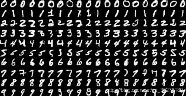
深度神经网络往往需要上百层,用上一节我们使用的直接通过weights矩阵来构建网络几乎不可能,所以需要pytorch的 nn 模块,为了演示它的用法, 我们将使用数据库MNIST。
每张图片都是28×28像素的
# Import necessary packages

%matplotlib inline  # 将 matplotlib 设置为以交互方式在 notebook 中工作
%config InlineBackend.figure_format = 'retina' #在分辨率较高的屏幕(例如 Retina 显示屏)上,notebook 中的默认图像可能会显得模糊。可以在 %matplotlib inline 之后使用 %config InlineBackend.figure_format = ‘retina’ 来呈现分辨率较高的图像。

import numpy as np
import torch
import helper #https://github.com/udacity/deep-learning-v2-pytorch/blob/master/intro-to-pytorch/helper.py
import matplotlib.pyplot as plt
下载数据
这里用的是torchvision包中的datasets模块,里面有MNIST的数据,可以下载。 transform是数据预处理,其中transforms.ToTensor()将图片的像素值range [0, 255] -> [0.0,1.0],transforms.Normalize(mean = (0.5, 0.5, 0.5), std = (0.5, 0.5, 0.5))再将数值进行正态化,均值和标准差分别是第一个括号里面的数字和第二个括号里面的数字,均值和标准差都是0.5的话可以把01的数值变成-11的数值。
### Run this cell

from torchvision import datasets, transforms

# Define a transform to normalize the data
transform = transforms.Compose([transforms.ToTensor(),
                              transforms.Normalize((0.5,), (0.5,)),
                              ])

# Download and load the training data
trainset = datasets.MNIST('~/.pytorch/MNIST_data/', download=True, train=True, transform=transform)
trainloader = torch.utils.data.DataLoader(trainset, batch_size=64, shuffle=True)
然后我们把训练数据load进trainloader,然后进行迭代iter(trainloader), 然后在每个loop里面对数据进行训练,就像这样:
for image, label in trainloader:
    ## do things with images and labels
图像是以size为(64, 1, 28, 28)的tensor储存的,其中64是batch的大小
.next()在这里就是不断调用并返回下一个值,参考链接
numpy.squeeze(a,axis = None)从数组的形状中删除单维度条目,即把shape中为1的维度去掉,axis若未指定则删除所有单维度的条目。通常在深度学习画图的时候用,因为直接用数组进行画图可能显示为空
dataiter = iter(trainloader)
images, labels = dataiter.next()
print(type(images))
print(images.shape)
print(labels.shape)
定义每层输入输出
我们现在见到的网络都是fully-conected或者dense,指的就是每一层的每个unit都和下一层的每个unit连接。在全连接的网络中,每层的输入都必须是一维的(这样才可以打包成为一个batch的2Dtensor),但是我们的图片是28x28 2D tensors, 必须先转化成1D的vectors。我们要把(64, 1, 28, 28) to转化成(64, 784)
Exercise: Flatten the batch of images images. Then build a multi-layer network with 784 input units, 256 hidden units, and 10 output units using random tensors for the weights and biases. For now, use a sigmoid activation for the hidden layer. Leave the output layer without an activation, we’ll add one that gives us a probability distribution next.
需要用到的function:
.view() 把原先tensor中的数据按照行优先的顺序排成一个一维的数据,然后按照参数组合成其他维度的tensor。参数-1就是自行计算
## Activation function
def activation(x):
    """ Sigmoid activation function
        Arguments
        ---------
        x: torch.Tensor
    """
    return 1/(1+torch.exp(-x))

 # Flatten the input images
inputs = images.view(images.shape[0],-1)

# Create parameters
W1 = torch.randn(784,256)
b1 = torch.randn(256)

W2 = torch.randn(256,10)
b2 = torch.randn(10)

h = activation(torch.mm(inputs,W1) + b1)
out = activation(torch.mm(h, w2) + b2)
一般情况:
## Your solution


## Activation function
def activation(x):
    """ Sigmoid activation function
        Arguments
        ---------
        x: torch.Tensor
    """
    return 1/(1+torch.exp(-x))

### Neural network
def multi_Layer_NW(inputUnits, hiddenUnits, outputUnits):
    torch.manual_seed(7) # Set the random seed so things are predictable

    # Define the size of each layer in our network
    n_input = inputUnits     # Number of input units, must match number of input features
    n_hidden = hiddenUnits   # Number of hidden units
    n_output = outputUnits   # Number of output units

    # Weights for inputs to hidden layer
    W1 = torch.randn(n_input, n_hidden)
    # Weights for hidden layer to output layer
    W2 = torch.randn(n_hidden, n_output)

    # and bias terms for hidden and output layers
    B1 = torch.randn((1, n_hidden))
    B2 = torch.randn((1, n_output))

    return W1,W2,B1,B2

def calc_output(features,W1,W2,B1,B2):
    h = activation(torch.matmul(features,W1).add_(B1))
    output = activation(torch.matmul(h,W2).add_(B2))
    return output

# Features are flattened batch input
features = torch.flatten(images,start_dim=1)
W1,W2,B1,B2 = multi_Layer_NW(features.shape[1],256,10)

out = calc_output(features,W1,W2,B1,B2) # output of your network, should have shape (64,10)
查看分类概率
通过softmax函数来查看每个数字所占的概率:
σ ( x i ) = e x i ∑ K k e x k \sigma(x_i) = \frac{e^{x_i}}{\textstyle\sum_{K}^k{e^{x_k}}} σ(xi)=∑Kkexkexi
注意在做矩阵除法的时候, tensor a with shape (64, 10) and a tensor b with shape (64,), doing a/b 会报错,因为pytorch会自动braodcast,会造成size mismatch,因此我们需要让b to have a shape of (64, 1)
def softmax(x):
    ## TODO: Implement the softmax function here
    return torch.exp(x)/torch.sum(torch.exp(x), dim=1).view(-1, 1)

# Here, out should be the output of the network in the previous excercise with shape (64,10)
probabilities = softmax(out)

# Does it have the right shape? Should be (64, 10)
print(probabilities.shape)
# Does it sum to 1?
print(probabilities.sum(dim=1))
构建网络
pytorch中的 nn模块可以方便的构建网络
下面是构建网络时会建的类,我们会一行一行的分析
class Network(nn.Module):
    def __init__(self):
        super().__init__()

        # Inputs to hidden layer linear transformation
        self.hidden = nn.Linear(784, 256)
        # Output layer, 10 units - one for each digit
        self.output = nn.Linear(256, 10)

        # Define sigmoid activation and softmax output
        self.sigmoid = nn.Sigmoid()
        self.softmax = nn.Softmax(dim=1)

    def forward(self, x):
        # Pass the input tensor through each of our operations
        x = self.hidden(x)
        x = self.sigmoid(x)
        x = self.output(x)
        x = self.softmax(x)

        return x
一点一点看:
class Network(nn.Module):
继承了nn.Module.,并且和super().__init__() 使用。
self.hidden = nn.Linear(784, 256)
这行建立了一个 linear transformation的模块, x W + b x\mathbf{W} + b xW+b有784个输入和256个输出,把它们assigns给 self.hidden. 这个module将会被用到后面的 forward 函数中。 当这个网络建立起来之后,有了weights和bias之后可以通过net.hidden.weight 和net.hidden.bias来访问weights和bias的tensor。
self.softmax = nn.Softmax(dim=1)
Setting dim=1 in nn.Softmax(dim=1) calculates softmax across the columns.
def forward(self, x):
PyTorch使用nn.Module必须要有一个 forward 函数定义。 它将x 作为输入然后经过在 __init__中定义的一系列操作。
x = self.hidden(x)
x = self.sigmoid(x)
x = self.output(x)
x = self.softmax(x)
在forward 函数中,x一个接一个的经过这些操作。
然后就可以建立Network 实例,可以打印出来看看它的文本表示
model = Network()
print (model)
'''
Network(
  (hidden): Linear(in_features=784, out_features=256, bias=True)
  (output): Linear(in_features=256, out_features=10, bias=True)
  (sigmoid): Sigmoid()
  (softmax): Softmax(dim=1)
)
'''
也可以使用torch.nn.functional,torch.nn.functional和torch.nn的区别链接
通常将import torch.nn.functional as F写成F
import torch.nn.functional as F

class Network(nn.Module):
    def __init__(self):
        super().__init__()
        # Inputs to hidden layer linear transformation
        self.hidden = nn.Linear(784, 256)
        # Output layer, 10 units - one for each digit
        self.output = nn.Linear(256, 10)

    def forward(self, x):
        # Hidden layer with sigmoid activation
        x = F.sigmoid(self.hidden(x))
        # Output layer with softmax activation
        x = F.softmax(self.output(x), dim=1)

        return x
激活函数
对激活函数的要求就是 The activation functions must be non-linear。这里是三个激活函数:

然后你按照下图的结构可以建立自己的网络
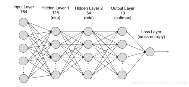
要求如下
Exercise: Create a network with 784 input units, a hidden layer with 128 units and a ReLU activation, then a hidden layer with 64 units and a ReLU activation, and finally an output layer with a softmax activation as shown above. You can use a ReLU activation with the
nn.ReLUmodule orF.relufunction.
这里是我的答案,仅供参考。
import torch.nn.functional as F

class MyNetwork(nn.Module):
    def __init__(self):
        super().__init__()
        self.fc1 = nn.Linear(784,128)
        self.fc2 = nn.Linear(128,64)
        self.output = nn.Linear(64,10)

    def forward(self,x):
        x = F.relu(self.fc1(x))
        x = F.relu(self.fc2(x))
        x = F.softmax(self.output(x), dim=1)

        return x

model = MyNetwork()
print (model)
初始化weights和bias
weights和bias自动初始化了,你可以通过 model.fc1.weight 来查看。
print(model.fc1.weight)
print(model.fc1.bias)

'''
Parameter containing:
tensor([[ 0.0074,  0.0126,  0.0136,  ..., -0.0305,  0.0031, -0.0169],
        [-0.0056, -0.0313,  0.0250,  ..., -0.0276, -0.0035, -0.0011],
        [-0.0059, -0.0284, -0.0092,  ...,  0.0146,  0.0092, -0.0347],
        ...,
        [-0.0227,  0.0313, -0.0265,  ..., -0.0280,  0.0268, -0.0074],
        [-0.0203,  0.0048,  0.0218,  ..., -0.0283,  0.0236, -0.0209],
        [-0.0037,  0.0138, -0.0274,  ...,  0.0268, -0.0338, -0.0260]],
       requires_grad=True)
Parameter containing:
tensor([-0.0285, -0.0111, -0.0321, -0.0245,  0.0211, -0.0246,  0.0001, -0.0341,
        -0.0258, -0.0197, -0.0157,  0.0031, -0.0341, -0.0336, -0.0139,  0.0004,
         0.0233,  0.0224, -0.0200,  0.0323,  0.0096, -0.0054, -0.0003, -0.0297,
         0.0311,  0.0010,  0.0088, -0.0158,  0.0205,  0.0158,  0.0315,  0.0085,
        -0.0243, -0.0132, -0.0239,  0.0058,  0.0026,  0.0080,  0.0260, -0.0191,
        -0.0356,  0.0034, -0.0335,  0.0233,  0.0279, -0.0070, -0.0074,  0.0322,
         0.0262, -0.0090, -0.0314, -0.0205, -0.0155, -0.0294,  0.0357, -0.0350,
        -0.0291,  0.0166,  0.0013,  0.0132, -0.0317,  0.0305, -0.0180, -0.0324,
         0.0264,  0.0306, -0.0005,  0.0178,  0.0242, -0.0183, -0.0020,  0.0176,
        -0.0194, -0.0265, -0.0244,  0.0306,  0.0338, -0.0276,  0.0281, -0.0272,
        -0.0111,  0.0127,  0.0270, -0.0086,  0.0199,  0.0308, -0.0144, -0.0003,
         0.0041, -0.0050, -0.0213, -0.0102,  0.0271, -0.0162, -0.0159, -0.0022,
        -0.0261,  0.0228,  0.0085, -0.0109,  0.0198,  0.0353,  0.0080,  0.0238,
         0.0114, -0.0234, -0.0075,  0.0019,  0.0192,  0.0333, -0.0166,  0.0226,
         0.0340,  0.0151, -0.0354,  0.0313, -0.0102, -0.0273, -0.0297, -0.0136,
        -0.0131, -0.0081, -0.0102, -0.0223,  0.0348,  0.0005, -0.0018, -0.0321],
       requires_grad=True)
'''
如果想要定制的初始化,也就是自己设置值,那么可以通过model.fc1.weight.data来访问并修改内容
# Set biases to all zeros
model.fc1.bias.data.fill_(0)
# sample from random normal with standard dev = 0.01
model.fc1.weight.data.normal_(std=0.01)
前向传播
现在已经拥有了网络,可以看看一张图片是如何pass这个网络的
# Grab some data
dataiter = iter(trainloader)
images, labels = dataiter.next()

# Resize images into a 1D vector, new shape is (batch size, color channels, image pixels)
images.resize_(64, 1, 784)
# or images.resize_(images.shape[0], 1, 784) to automatically get batch size

# Forward pass through the network
img_idx = 0
ps = model.forward(images[img_idx,:])

img = images[img_idx]
helper.view_classify(img.view(1, 28, 28), ps)
使用nn.Sequential
PyTorch提供了一个更方便的建立网络的方法,tensor可以序列的经过一系列操作,就是nn.Sequential (documentation)。方法如下:
# Hyperparameters for our network
input_size = 784
hidden_sizes = [128, 64]
output_size = 10
# Build a feed-forward network
model = nn.Sequential(nn.Linear(input_size, hidden_sizes[0]),
nn.ReLU(),
nn.Linear(hidden_sizes[0], hidden_sizes[1]),
nn.ReLU(),
nn.Linear(hidden_sizes[1], output_size),
nn.Softmax(dim=1))
print(model)
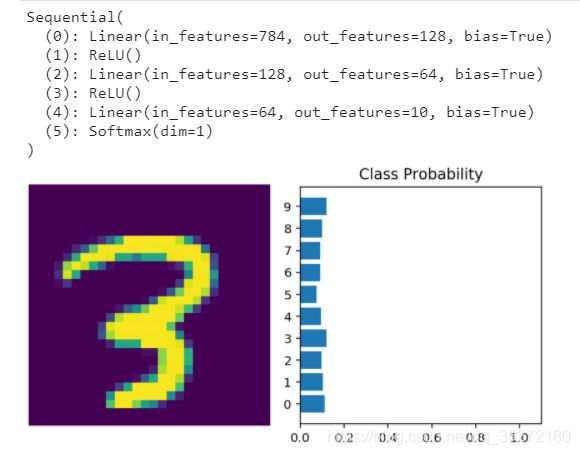
# Forward pass through the network and display output
images, labels = next(iter(trainloader))
images.resize_(images.shape[0], 1, 784)
ps = model.forward(images[0,:])
helper.view_classify(images[0].view(1, 28, 28), ps)
输出:
如果你想要查看第一个先行操作的weights,可以使用model[0]
print(model[0])
model[0].weight
'''

Linear(in_features=784, out_features=128, bias=True)


[40]:
Parameter containing:
tensor([[ 0.0157, -0.0145, -0.0135,  ..., -0.0243,  0.0220, -0.0318],
        [-0.0314,  0.0171, -0.0275,  ...,  0.0243,  0.0197,  0.0089],
        [-0.0225, -0.0105,  0.0196,  ...,  0.0015, -0.0318, -0.0037],
        ...,
        [ 0.0273,  0.0232, -0.0140,  ..., -0.0142,  0.0127,  0.0232],
        [ 0.0194, -0.0251, -0.0067,  ...,  0.0258, -0.0152,  0.0220],
        [-0.0106, -0.0298, -0.0295,  ..., -0.0226, -0.0099, -0.0019]],
       requires_grad=True)

'''
或者你也可以通过OrderedDict来给每一层命名,这是一个字典型的数据,每个keys名都必须是不重复的。
from collections import OrderedDict
model = nn.Sequential(OrderedDict([
                      ('fc1', nn.Linear(input_size, hidden_sizes[0])),
                      ('relu1', nn.ReLU()),
                      ('fc2', nn.Linear(hidden_sizes[0], hidden_sizes[1])),
                      ('relu2', nn.ReLU()),
                      ('output', nn.Linear(hidden_sizes[1], output_size)),
                      ('softmax', nn.Softmax(dim=1))]))
print (model)
'''
Sequential(
  (fc1): Linear(in_features=784, out_features=128, bias=True)
  (relu1): ReLU()
  (fc2): Linear(in_features=128, out_features=64, bias=True)
  (relu2): ReLU()
  (output): Linear(in_features=64, out_features=10, bias=True)
  (softmax): Softmax(dim=1)
)
'''
现在再访问这一层就可以用model.fc1
print(model[0])
print(model.fc1)
'''
Linear(in_features=784, out_features=128, bias=True)
Linear(in_features=784, out_features=128, bias=True)
'''
总结
在正式训练之前,我们需要做的工作有:
- 下载数据,load数据,对数据进行预处理。需要用到的函数:
torchvision.datasets,torchvision.transforms.Compose,torch.utils.data.DataLoader - 建立迭代,对训练图片建立迭代,以batch的方式送入网络。需要用到的函数:
iter(trainloader),.next() - . build networks构建网络,定义每一层输入输出的维度,构建forward函数。需要用到的函数:
torch.nn,torch.nn.functional
以上两个步骤中需要用到的其他功能:
- 访问某一层:
model[0]或者model.fc1. - 访问某一层的weights和bias:
model.fc1.weight,model.fc1.bias
查看完整代码参考
https://github.com/udacity/deep-learning-v2-pytorch.git中
intro-to-pytorch的Part 2
本系列笔记来自Udacity课程《Intro to Deep Learning with Pytorch》
全部笔记请关注微信公众号【阿肉爱学习】,在菜单栏点击“利其器”,并选择“pytorch”查看