吴恩达深度学习第一课-第二周笔记及课后编程题

逻辑回归（Logistic Regression）

逻辑回归用于二分类（Binary Classification），输出值为0-1范围内的实数。

通常规定：输出值小于0.5分类为"0"，输出值大于0.5分类为"1"

逻辑分布（Logistic Distribution）

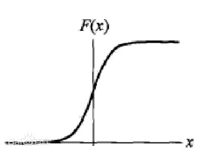
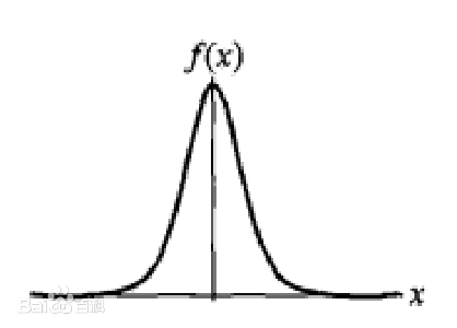
逻辑分布为连续型概率分布。

分布函数：

密度函数：

可见f(x)与正态分布形状相似，不过尾部更长，波峰更高，在数据分布情况如此时，选择逻辑分布建模比正态分布更合适。

Sigmoid Function

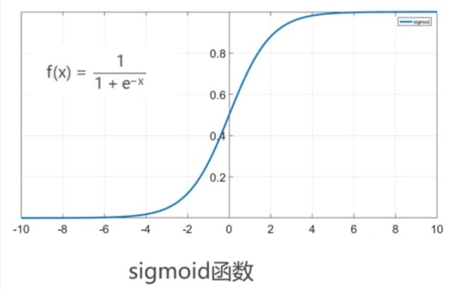
当μ=0，γ=1时，称为标准逻辑分布，即 ，该函数也称为Sigmoid函数，是逻辑回归的关键。

由图像可知，当x趋向+∞时，输出值趋向1；反之，当x趋向-∞时，输出值趋向0。即Sigmoid函数的输出范围为(0,1)。

通常Sigmoid函数表示为：，它的导数可以用自身表示，即：。

Why sigmoid？

线性模型 ，显然不符合二分类问题的输出要求（即0-1范围内的实数），所以需要使用广义的线性模型，针对输出要求，对数几率函数是符合的。

几率（odds）：事件发生与不发生的概率比值。

令y表示正例（即“1”）的概率，1-y表示反例（即“0”）的概率。

对数几率函数： ，即 ①

由①可得：

损失函数（Loss/Cost Function）

估计值 ，其中

当我们使用最小二乘 计算误差，使用梯度下降法（Gradient Descent）无法收敛，所以舍弃这种方法，转而使用最小化交叉熵（Cross Entropy），原因如下：

逻辑回归的本质：假设数据服从逻辑分布，然后用最大似然估计（Maximum Likelyhood Estimation, MLE）做参数的估计。

逻辑回归在单个样本上的概率为

• 当y=1，

• 当y=0，

似然函数为 ②

对③两边取对数得 ③

因为对数函数是严格单调递增函数，所以求最大似然估计的对数（③）等同于求最大似然估计（②），而求最大似然估计的对数等同于求最小负的最大似然估计对数，即最小交叉熵。

Loss Function

通常用于衡量模型在单个训练样本上的表现

Cost Function

通常用于衡量模型在全部训练样本上的表现

梯度下降（Gradient Descent）

沿梯度下降的方向求解极小值（也可以沿梯度上升方向求解极大值）

重复进行：

• 

• 

直到J(w,b)收敛到全局最小值（global minimum）

注：

• α为学习率，决定每一步下降的步幅，是一个大于0的实数

• 为J(w,b)在w方向上的斜率

• 为J(w,b)在b方向上的斜率

单个训练样本的前向传播与反向传播

前向传播（Forward Propagation）

给定 :

,

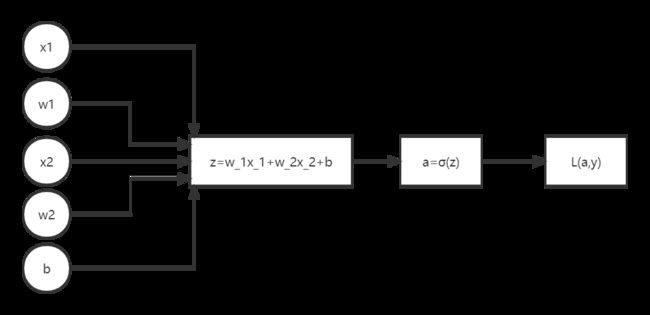
前向传播图：

反向传播（Back Propagation）

我们规定: ， 如

对前向传播图由后往前做反向传播，即逐步往回求导：

梯度下降：

重复上述的前向与反向传播，直到损失函数J(w,b)收敛到全局最小值

多个训练样本的前向传播与反向传播

给定：

For循环

伪代码如下：

J = dw1 = dw2 = db = 0
for i=1 to m:
    z[i] = w^T*x[i]+b
    a[i] = σ(z[i])
    J += -[y[i]loga[i]+(1-y[i])log(1-a[i])]
    dz[i] = a[i]-y[i]
    dw1 += x[i][0]dz[i]
    dw2 += x[i][1]dz[i]
    db += dz[i]
J /= m
dw1 /= m
dw2 /= m
b /= m
w1 -= αdw1
w2 -= αdw2
b -= αdb

重复上述步骤直到J(w,b)收敛到全局最小值

向量化（Vectorization）

在数据集稍大一些的情况下For循环已经会很慢，而向量化会更快且代码更简洁

z = np.dot(w.T,X)+b
A = σ(Z)
dz = A-Y
dw = (1/m)*np.dot(X,dz.T)
db = (1/m)*np.sum(dz)
w -= αdw
b -= αdb

重复上述步骤直到J(w,b)收敛到全局最小值

课后编程题

注：在完成编程题前，要先下载两个重要文件（缺一不可）：

• lr_utils.py

• datasets

下载链接：第二周课后编程题资料，提取码：r5ra

完整代码如下：

注：

• 题目以及每一道小题的提示均以#注释方式在代码中呈现

• 逐小题进行编写和运行效果更加，即模仿Jupyter Notebook的代码块形式进行编写与运行

"""
Purpose:
build a Logistic Regression classifier to recognize cats

Learn to build the general architecture of a learning algorithm, including:
- Initializing parameters
- Calculating the cost function and its gradient
- Using an optimization algorithm (gradient descent)
"""

import numpy as np
import matplotlib.pyplot as plt
import scipy
from scipy import ndimage
from lr_utils import load_dataset

# 加载数据到程序中
train_set_x_orig, train_set_y, test_set_x_orig, test_set_y, classes = load_dataset()
# 查看训练集某张图片
index = 7  # 可以根据自己的想法更换index，查看不同的图片
plt.imshow(train_set_x_orig[index])
# 使用np.squeeze的目的是压缩维度，未压缩的“train_set_y[:, index]”值为[1]，压缩后的“train_set_y[:, index]”值为1
# 只有压缩后的值才能进行解码操作
print("y = " + str(train_set_y[:, index]) + ", it's a '" + classes[np.squeeze(train_set_y[:, index])].decode("utf-8") +
      "' picture")

# Exercise1:Find the values for: - m_train (number of training examples) - m_test (number of test examples)
# - num_px (= height = width of a training image)
# Remember that train_set_x_orig is a numpy-array of shape (m_train, num_px, num_px, 3). For instance, you can access
# m_train by writing train_set_x_orig.shape[0].

# ## START CODE HERE ## (≈ 3 lines of code)
m_train = train_set_y.shape[1]
m_test = test_set_y.shape[1]
num_px = train_set_x_orig.shape[1]
# ## END CODE HERE ##

print("Number of training examples: m_train = " + str(m_train))
print("Number of testing examples: m_test = " + str(m_test))
print("Height/Width of each image: num_px = " + str(num_px))
print("Each image is of size: (" + str(num_px) + ", " + str(num_px) + ", 3)")
print("train_set_x shape: " + str(train_set_x_orig.shape))
print("train_set_y shape: " + str(train_set_y.shape))
print("test_set_x shape: " + str(test_set_x_orig.shape))
print("test_set_y shape: " + str(test_set_y.shape))

# Exercise2: Reshape the training and test data sets so that images of size (num_px, num_px, 3) are flattened into
# single vectors of shape (num_px*num_px* 3, 1).
# A trick when you want to flatten a matrix X of shape (a,b,c,d) to a matrix X_flatten of shape (b*c*d, a) is to use:
# X_flatten = X.reshape(X.shape[0], -1).T

# ## START CODE HERE ## (≈ 2 lines of code)
train_set_x_flatten = train_set_x_orig.reshape(train_set_x_orig.shape[0], -1).T
test_set_x_flatten = test_set_x_orig.reshape(test_set_x_orig.shape[0], -1).T
# ## END CODE HERE ##

print("train_set_x_flatten shape: " + str(train_set_x_flatten.shape))
print("train_set_y shape: " + str(train_set_y.shape))
print("test_set_x_flatten shape: " + str(test_set_x_flatten.shape))
print("test_set_y shape: " + str(test_set_y.shape))
print("sanity check after reshaping: " + str(train_set_x_flatten[0:5, 0]))

"""
One common preprocessing step in machine learning is to center and standardize your dataset, meaning that you substract
the mean of the whole numpy array from each example, and then divide each example by the standard deviation of the whole 
numpy array.
But for picture datasets, it is simpler and more convenient and works almost as well to just divide every row of the 
dataset by 255 (the maximum value of a pixel channel).
"""
train_set_x = train_set_x_flatten / 255
test_set_x = test_set_x_flatten / 255


"""
The main steps for building a Neural Network are:
1.Define the model structure (such as number of input features)
2.Initialize the model's parameters
3.Loop:
    - Calculate current loss (forward propagation)
    - Calculate current gradient (backward propagation)
    - Update parameters (gradient descent)
You often build 1-3 separately and integrate them into one function we call model()
"""
# Exercise3: "sigmoid()" function
def sigmoid(z):
    """
        Compute the sigmoid of z

        Arguments:
        x -- A scalar or numpy array of any size.

        Return:
        s -- sigmoid(z)
    """

    # ## START CODE HERE ## (≈ 1 line of code)
    s = 1 / (1 + np.exp(-z))
    # ## END CODE HERE ##

    return s


print("-----------sigmoid test---------------")
print("sigmoid(0) = " + str(sigmoid(0)))
print("sigmoid(9.2) = " + str(sigmoid(9.2)))


# Exercise4: Implement parameter initialization in the cell below. You have to initialize w as a vector of zeros. If you
# don't know what numpy function to use, look up np.zeros() in the Numpy library's documentation.

# GRADED FUNCTION: initialize_with_zeros
def initialize_with_zeros(dim):
    """
    This function creates a vector of zeros of shape (dim, 1) for w and initializes b to 0.

    Argument:
    dim -- size of the w vector we want (or number of parameters in this case)

    Returns:
    w -- initialized vector of shape (dim, 1)
    b -- initialized scalar (corresponds to the bias)
    """
    # ## START CODE HERE ## (≈ 1 line of code)
    w = np.zeros(shape=(dim, 1))
    b = 0
    # ## END CODE HERE ##

    assert (w.shape == (dim, 1))
    assert (isinstance(b, float) or isinstance(b, int))
    return w, b

# For image inputs, w will be of shape (num_px * num_px * 3, 1)


# Exercise5: Implement a function propagate() that computes the cost function and its gradient

# GRADED FUNCTION: propagate
def propagate(w, b, X, Y):
    """
        Implement the cost function and its gradient for the propagation explained above

        Arguments:
        w -- weights, a numpy array of size (num_px * num_px * 3, 1)
        b -- bias, a scalar
        X -- data of size (num_px * num_px * 3, number of examples)
        Y -- true "label" vector (containing 0 if non-cat, 1 if cat) of size (1, number of examples)

        Return:
        cost -- negative log-likelihood cost for logistic regression
        dw -- gradient of the loss with respect to w, thus same shape as w
        db -- gradient of the loss with respect to b, thus same shape as b

        Tips:
        - Write your code step by step for the propagation
    """
    m = X.shape[1]  # amount of samples

    # FORWARD PROPAGATION (FROM X TO COST)

    # ## START CODE HERE ## (≈ 2 lines of code)
    A = sigmoid(np.dot(w.T, X) + b)  # compute activation
    cost = (- 1 / m) * np.sum(Y * np.log(A) + (1 - Y) * (np.log(1 - A)))  # compute cost
    # ## END CODE HERE ##

    # BACKWARD PROPAGATION (TO FIND GRAD)

    # ## START CODE HERE ## (≈ 2 lines of code)
    dw = (1/m) * np.dot(X, (A-Y).T)
    db = (1/m) * np.sum(A-Y)
    # ## END CODE HERE ##

    assert(dw.shape == w.shape)
    assert(db.dtype == float)
    cost = np.squeeze(cost)  # squeeze作用：从数组的形状中删除单维度条目，即把shape为1的维度去掉
    assert(cost.shape == ())
    # 创建一个字典，把dw和db保存起来
    grads = {"dw": dw,
             "db": db}
    return grads, cost


print("-----------propagate test---------------")
w, b, X, Y = np.array([[1], [2]]), 2, np.array([[1, 2], [3, 4]]), np.array([[1, 0]])
grads, cost = propagate(w, b, X, Y)
print("dw = " + str(grads["dw"]))
print("db = " + str(grads["db"]))
print("cost = " + str(cost))


# Exercise6:Write down the optimization function. The goal is to learn w and b by minimizing the cost function J.
# For a parameter θ , the update rule is θ - αdθ, where α is the learning rate.

# GRADED FUNCTION: optimize
def optimize(w, b, X, Y, num_iterations, learning_rate, print_cost=False):
    """
    This function optimizes w and b by running a gradient descent algorithm

    Arguments:
    w -- weights, a numpy array of size (num_px * num_px * 3, 1)
    b -- bias, a scalar
    X -- data of shape (num_px * num_px * 3, number of examples)
    Y -- true "label" vector (containing 0 if non-cat, 1 if cat), of shape (1, number of examples)
    num_iterations -- number of iterations of the optimization loop
    learning_rate -- learning rate of the gradient descent update rule
    print_cost -- True to print the loss every 100 steps

    Returns:
    params -- dictionary containing the weights w and bias b
    grads -- dictionary containing the gradients of the weights and bias with respect to the cost function
    costs -- list of all the costs computed during the optimization, this will be used to plot the learning curve.

    Tips:
    You basically need to write down two steps and iterate through them:
        1) Calculate the cost and the gradient for the current parameters. Use propagate().
        2) Update the parameters using gradient descent rule for w and b.
    """

    costs = []

    for i in range(num_iterations):
        # Cost and gradient calculation (≈ 1-4 lines of code)
        # ## START CODE HERE ##
        grads, cost = propagate(w, b, X, Y)
        # ## END CODE HERE ##

        # Retrieve derivatives from grads
        dw = grads["dw"]
        db = grads["db"]

        # update rule (≈ 2 lines of code)
        # ## START CODE HERE ##
        w = w - learning_rate * dw
        b = b - learning_rate * db
        # ## END CODE HERE ##

        # Record the costs
        if i % 100 == 0:
            costs.append(cost)

        # Print the cost every 100 training examples
        if print_cost and (i % 100 == 0):
            print("Cost after iteration %i: %f" % (i, cost))

    params = {"w": w,
              "b": b}
    grads = {"dw": dw,
             "db": db}
    return params, grads, costs


print("-----------optimize test---------------")
w, b, X, Y = np.array([[1], [2]]), 2, np.array([[1, 2], [3, 4]]), np.array([[1, 0]])
params, grads, costs = optimize(w, b, X, Y, num_iterations=100, learning_rate=0.009, print_cost=False)
print("w = " + str(params["w"]))
print("b = " + str(params["b"]))
print("dw = " + str(grads["dw"]))
print("db = " + str(grads["db"]))


# Exercise7: The previous function will output the learned w and b. We are able to use w and b to predict the labels for
# a dataset X. Implement the predict() function. There is two steps to computing predictions:
# 1. Calculate Yhat = A = sigmoid(w.T*X + b)
# 2. Convert the entries of a into 0 (if activation <= 0.5) or 1 (if activation > 0.5), stores the predictions in a
# vector Y_prediction. If you wish, you can use an if/else statement in a for loop (though there is also a way to
# vectorize this).

# GRADED FUNCTION: predict

def predict(w, b, X):
    """
    Predict whether the label is 0 or 1 using learned logistic regression parameters (w, b)

    Arguments:
    w -- weights, a numpy array of size (num_px * num_px * 3, 1)
    b -- bias, a scalar
    X -- data of size (num_px * num_px * 3, number of examples)

    Returns:
    Y_prediction -- a numpy array (vector) containing all predictions (0/1) for the examples in X
    """
    m = X.shape[1]
    Y_prediction = np.zeros((1, m))
    w = w.reshape(X.shape[0], 1)

    # Compute vector "A" predicting the probabilities of a cat being present in the picture
    # ## START CODE HERE ## (≈ 1 line of code)
    A = sigmoid(np.dot(w.T, X) + b)
    # ## END CODE HERE ##

    for i in range(A.shape[1]):
        # Convert probabilities a[0,i] to actual predictions p[0,i]
        # ## START CODE HERE ## (≈ 4 lines of code)
        Y_prediction[0, i] = 1 if A[0, i] > 0.5 else 0
        # ## END CODE HERE ##

    assert(Y_prediction.shape == (1, m))

    return Y_prediction


print("-----------predict test---------------")
w, b, X, Y = np.array([[1], [2]]), 2, np.array([[1, 2], [3, 4]]), np.array([[1, 0]])
print("predictions = " + str(predict(w, b, X)))


# You will now see how the overall model is structured by putting together all the building blocks (functions
# implemented in the previous parts) together, in the right order.

# Exercise8: Implement the model function. Use the following notation: - Y_prediction for your predictions on the test
# set - Y_prediction_train for your predictions on the train set - w, costs, grads for the outputs of optimize()

def model(X_train, Y_train, X_test, Y_test, num_iterations=2000, learning_rate=0.5, print_cost=False):
    """
    Builds the logistic regression model by calling the function you've implemented previously

    Arguments:
    X_train -- training set represented by a numpy array of shape (num_px * num_px * 3, m_train)
    Y_train -- training labels represented by a numpy array (vector) of shape (1, m_train)
    X_test -- test set represented by a numpy array of shape (num_px * num_px * 3, m_test)
    Y_test -- test labels represented by a numpy array (vector) of shape (1, m_test)
    num_iterations -- hyperparameter representing the number of iterations to optimize the parameters
    learning_rate -- hyperparameter representing the learning rate used in the update rule of optimize()
    print_cost -- Set to true to print the cost every 100 iterations

    Returns:
    d -- dictionary containing information about the model.
    """

    # ## START CODE HERE ##
    # initialize parameters with zeros (≈ 1 line of code)
    w, b = initialize_with_zeros(X_train.shape[0])

    # Gradient descent (≈ 1 line of code)
    parameters, grads, costs = optimize(w, b, X_train, Y_train, num_iterations, learning_rate, print_cost)

    # Retrieve parameters w and b from dictionary "parameters"
    w = parameters["w"]
    b = parameters["b"]

    # Predict test/train set examples (≈ 2 lines of code)
    Y_prediction_test = predict(w, b, X_test)
    Y_prediction_train = predict(w, b, X_train)
    # ## END CODE HERE ##

    # Print train/test Errors
    print("train accuracy: {} %".format(100 - np.mean(np.abs(Y_prediction_train - Y_train)) * 100))
    print("test accuracy: {} %".format(100 - np.mean(np.abs(Y_prediction_test - Y_test)) * 100))

    d = {"costs": costs,
         "Y_prediction_test": Y_prediction_test,
         "Y_prediction_train": Y_prediction_train,
         "w": w,
         "b": b,
         "learning_rate": learning_rate,
         "num_iterations": num_iterations}

    return d


d = model(train_set_x, train_set_y, test_set_x, test_set_y, num_iterations=2000, learning_rate=0.005, print_cost= True)

"""
Comment: Training accuracy is close to 100%. This is a good sanity check: your model is working and has high enough 
capacity to fit the training data. Test error is 68%. It is actually not bad for this simple model, given the small 
dataset we used and that logistic regression is a linear classifier. But no worries, you'll build an even better 
classifier next week!

Also, you see that the model is clearly overfitting the training data. Later in this specialization you will learn how 
to reduce overfitting, for example by using regularization.
"""

# Plot learning curve (with costs)
costs = np.squeeze(d['costs'])
plt.plot(costs)
plt.ylabel('cost')
plt.xlabel('iterations (per hundreds)')
plt.title("Learning rate =" + str(d["learning_rate"]))
plt.show()
# Interpretation: You can see the cost decreasing. It shows that the parameters are being learned. However, you see that
# you could train the model even more on the training set. Try to increase the number of iterations in the cell above
# and rerun the cells. You might see that the training set accuracy goes up, but the test set accuracy goes down. This
# is called overfitting.


"""
Reminder: In order for Gradient Descent to work you must choose the learning rate wisely. The learning rate 
determines how rapidly we update the parameters. If the learning rate is too large we may "overshoot" the optimal 
value. Similarly, if it is too small we will need too many iterations to converge to the best values. That's why it is
crucial to use a well-tuned learning rate.
"""
learning_rates = [0.01, 0.001, 0.0001]
models = {}
for i in learning_rates:
    print("learning rate is: " + str(i))
    models[str(i)] = model(train_set_x, train_set_y, test_set_x, test_set_y, num_iterations=1500, learning_rate=i,
                           print_cost=False)
    print('\n' + "-------------------------------------------------------" + '\n')

for i in learning_rates:
    plt.plot(np.squeeze(models[str(i)]["costs"]), label=str(models[str(i)]["learning_rate"]))

plt.ylabel('cost')
plt.xlabel('iterations')

legend = plt.legend(loc='upper center', shadow=True)
frame = legend.get_frame()
frame.set_facecolor('0.90')
plt.show()
"""
Interpretation:

- Different learning rates give different costs and thus different predictions results.
- If the learning rate is too large (0.01), the cost may oscillate up and down. It may even diverge (though in this 
  example, using 0.01 still eventually ends up at a good value for the cost).
- A lower cost doesn't mean a better model. You have to check if there is possibly overfitting. It happens when the 
  training accuracy is a lot higher than the test accuracy.
- In deep learning, we usually recommend that you:
    - Choose the learning rate that better minimizes the cost function.
    - If your model overfits, use other techniques to reduce overfitting.
"""

# optional
# Test model with your own image
# ## START CODE HERE ## (PUT YOUR IMAGE NAME)
my_image = "my_image.jpg"   # change this to the name of your image file
# ## END CODE HERE ##

# We preprocess the image to fit your algorithm.
fname = "images/" + my_image
image = np.array(ndimage.imread(fname, flatten=False))
my_image = scipy.misc.imresize(image, size=(num_px, num_px)).reshape((1, num_px * num_px * 3)).T
my_predicted_image = predict(d["w"], d["b"], my_image)

plt.imshow(image)
print("y = " + str(np.squeeze(my_predicted_image)) + ", your algorithm predicts a \"" +
      classes[np.squeeze(train_set_y[:, index])].decode("utf-8"))

有几个重要的点：

• 为了方便，我们要把维度为（64，64，3）的numpy数组重新构造为（64 x 64 x 3，1）的数组，要乘以3的原因是每张图片是由64x64像素构成的，而每个像素点由（R，G，B）三原色构成的，所以要乘以3。在此之后，我们的训练和测试数据集是一个numpy数组，【每列代表一个平坦的图像】

• 机器学习中一个常见的预处理步骤是对数据集进行居中和标准化，这意味着可以减去每个示例中整个numpy数组的平均值，然后将每个示例除以整个numpy数组的标准偏差。但对于图片数据集，它更简单，更方便，几乎可以将数据集的每一行除以255（像素通道的最大值），因为在RGB中不存在比255大的数据，所以我们可以放心的除以255，让标准化的数据位于[0,1]之间

• 建立神经网络的主要步骤是：

1、定义模型结构（例如输入特征的数量）

2、初始化模型的参数

3、循环：

3.1 计算当前损失（前向传播）

3.2 计算当前梯度（反向传播）

3.3 更新参数（梯度下降）

我们经常将1-3分开编写，然后将它们整合到一个新的函数：model()中

• 我们更改一下学习率和迭代次数，有可能会发现训练集的准确性可能会提高，但是测试集准确性会下降，这是由于过拟合造成的，但是我们并不需要担心，我们以后会使用更好的算法来解决这些问题的。

• 为了让梯度下降起作用，我们必须明智地选择学习率。学习率 α 决定了我们更新参数的速度。如果学习率过高，我们可能会“超过”最优值。同样，如果它太小，我们将需要更多迭代才能收敛到最佳值。这就是为什么使用良好调整的学习率至关重要的原因。

参考

【吴恩达课后编程作业】Course 1 - 神经网络和深度学习 - 第二周作业

Logistic Regression with a Neural Network mindset

【机器学习】逻辑回归（非常详细）

百度百科-最大似然估计

百度百科-交叉熵