Scikit-network-09：Classification

Classification

PageRank

介绍基于Pagerank的图节点的分类，该节点基于几个节点的标签。

from IPython.display import SVG
import numpy as np

from sknetwork.data import karate_club, painters, movie_actor
from sknetwork.classification import PageRankClassifier
from sknetwork.visualization import svg_graph, svg_digraph, svg_bigraph

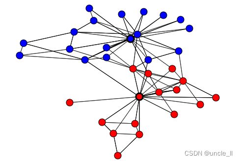
图

graph = karate_club(metadata=True)
adjacency = graph.adjacency
position = graph.position
labels_true = graph.labels
labels_true

array([1, 1, 1, 1, 1, 1, 1, 1, 1, 0, 1, 1, 1, 1, 0, 0, 1, 1, 0, 1, 0, 1,
       0, 0, 0, 0, 0, 0, 0, 0, 0, 0, 0, 0])

seeds = {i: labels_true[i] for i in [0, 33]}
pagerank = PageRankClassifier()
labels_pred = pagerank.fit_transform(adjacency, seeds)
labels_pred

array([1, 1, 1, 1, 1, 1, 1, 1, 0, 0, 1, 1, 1, 1, 0, 0, 1, 1, 0, 1, 0, 1,
       0, 0, 0, 0, 0, 0, 0, 0, 0, 0, 0, 0])

precision = np.round(np.mean(labels_pred==labels_true), 2)
precision
# 0.97
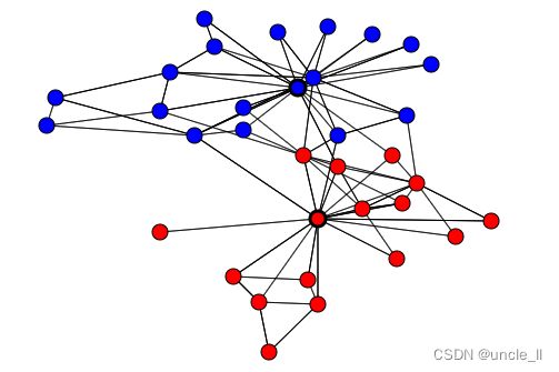
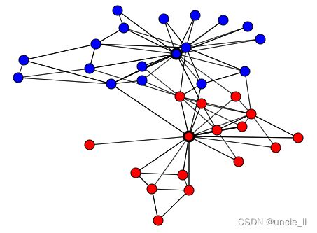
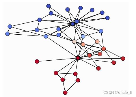
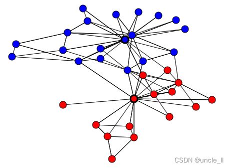
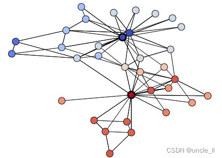
image = svg_graph(adjacency, position, labels=labels_pred, seeds=seeds)
SVG(image)

# soft classification (here probability of label 1)
label = 1
membership = pagerank.membership_
scores = membership[:,label].toarray().ravel()
print(scores)

[0.85083397 0.67169185 0.53881723 0.71812199 0.86360047 0.86708137
 0.86708137 0.72814855 0.453558   0.28963328 0.86360047 0.85626903
 0.80825129 0.57509049 0.18758663 0.18758663 0.87180985 0.79336306
 0.18758663 0.54964922 0.18758663 0.79336306 0.18758663 0.21970262
 0.33534748 0.31974366 0.16306381 0.28127132 0.32151073 0.18639406
 0.35142577 0.40884207 0.25890729 0.15608262]

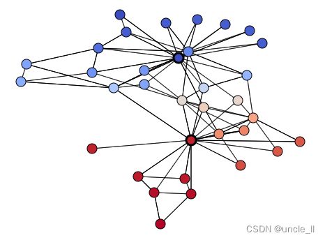
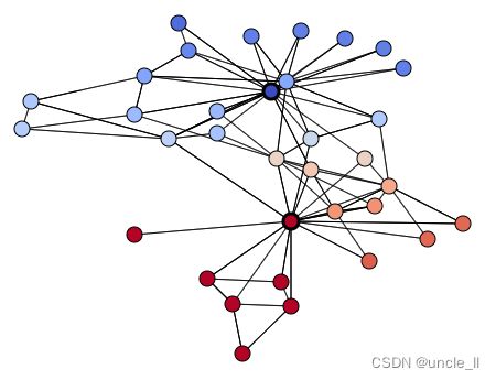
image = svg_graph(adjacency, position, scores=scores, seeds=seeds)
SVG(image)

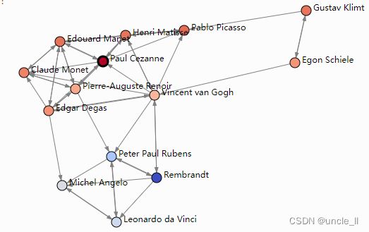
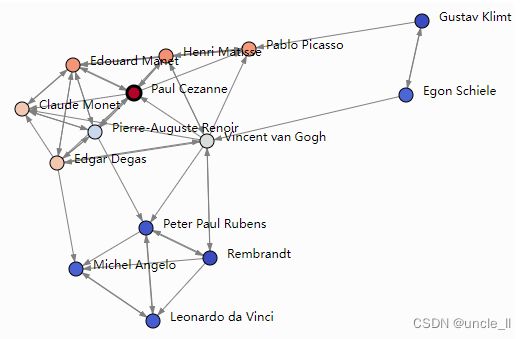
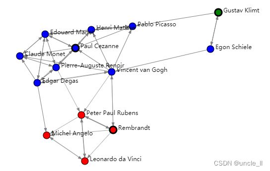
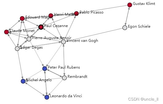
有向图

graph = painters(metadata=True)
adjacency = graph.adjacency
position = graph.position
names = graph.names

rembrandt = 5
klimt = 6
cezanne = 11
seeds = {cezanne: 0, rembrandt: 1, klimt: 2}

pagerank = PageRankClassifier()
labels = pagerank.fit_transform(adjacency, seeds)
labels
# array([2, 0, 1, 0, 1, 1, 2, 0, 2, 1, 0, 0, 0, 2])

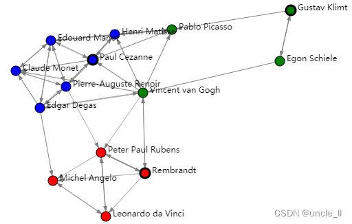
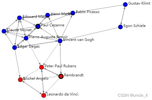
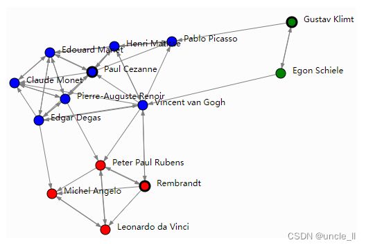
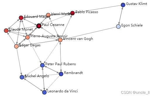
image = svg_digraph(adjacency, position, names, labels=labels, seeds=seeds)
SVG(image)

# soft classification
membership = pagerank.membership_
scores = membership[:, 0].toarray().ravel()
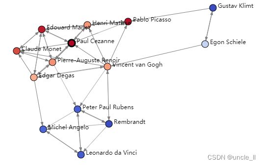
image = svg_digraph(adjacency, position, names, scores=scores, seeds=[cezanne])
SVG(image)

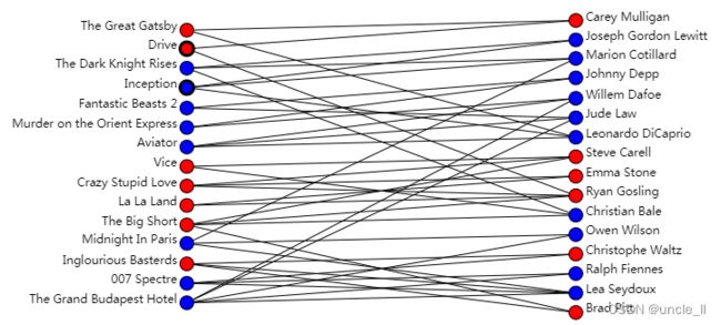
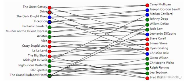
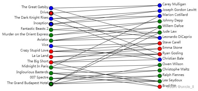
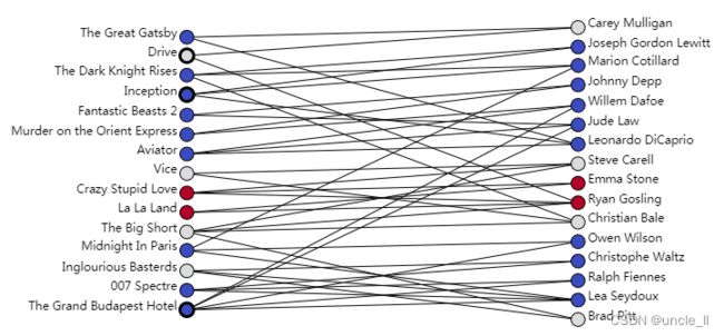
二部图

graph = movie_actor(metadata=True)
biadjacency = graph.biadjacency
names_row = graph.names_row
names_col = graph.names_col

inception = 0
drive = 3
budapest = 8

pagerank = PageRankClassifier()
pagerank.fit(biadjacency, seeds_row)
labels_row = pagerank.labels_row_
labels_col = pagerank.labels_col_

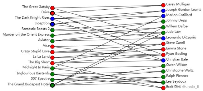
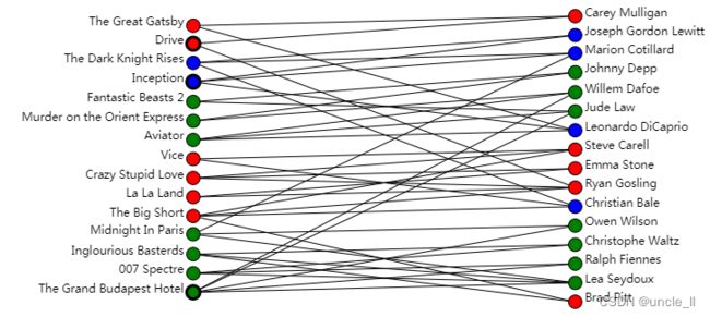
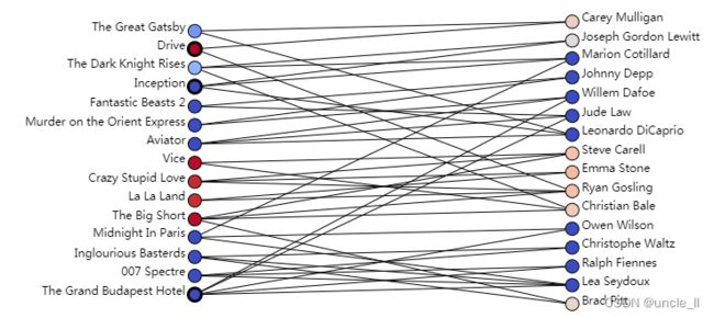
image = svg_bigraph(
    biadjacency, names_row, names_col, labels_row, labels_col, seeds_row=seeds_row)

SVG(image)

# soft classification
membership_row = pagerank.membership_row_
membership_col = pagerank.membership_col_

label = 1
scores_row = membership_row[:,label].toarray().ravel()
scores_col = membership_col[:,label].toarray().ravel()

image = svg_bigraph(biadjacency, names_row, names_col, scores_row=scores_row, scores_col=scores_col,
                    seeds_row=seeds_row)
SVG(image)

---

Diffusion

扩散算法是一种数据处理方法，目的在于通过扩散处理使得元素之间相互影响，从而实现完全的雪崩效应。

from IPython.display import SVG
import numpy as np
from sknetwork.data import karate_club, painters, movie_actor
from sknetwork.classification import DiffusionClassifier
from sknetwork.visualization import svg_graph, svg_digraph, svg_bigraph

图

graph = karate_club(metadata=True)
adjacency = graph.adjacency
position = graph.position
labels_true = graph.labels

seeds = {i: labels_true[i] for i in [0, 33]}
diffusion = DiffusionClassifier()
labels_pred = diffusion.fit_transform(adjacency, seeds)
labels_pred
# [1, 1, 0, 1, 1, 1, 1, 1, 0, 0, 1, 1, 1, 1, 0, 0, 1, 1, 0, 1, 0, 1, 0, 0, 0, 0, 0, 0, 0, 0, 0, 0, 0, 0]

precision = np.round(np.mean(labels_pred==labels_true), 2)
precision
# 0.94

image = svg_graph(adjacency, position, labels=labels_pred, seeds=seeds)
SVG(image)

# soft classification (here probability of label 1)
scores = diffusion.score(label=1)
image = svg_graph(adjacency, position, scores=scores, seeds=seeds)
SVG(image)

有向图

graph = painters(metadata=True)
adjacency = graph.adjacency
position = graph.position
names = graph.names

rembrant = 5
cezanne = 11
seeds = {cezanne: 0, rembrant: 1}

diffusion = DiffusionClassifier()
labels = diffusion.fit_transform(adjacency, seeds)

image = svg_digraph(adjacency, position, names, labels=labels, seeds=seeds)
SVG(image)

# soft classification (here probability of label 0)
scores = diffusion.score(label=0)
image = svg_digraph(adjacency, position, names=names, scores=scores, seeds=[cezanne])
SVG(image)

二部图

graph = movie_actor(metadata=True)
biadjacency = graph.biadjacency
names_row = graph.names_row
names_col = graph.names_col

inception = 0
drive = 3
seeds_row = {inception: 0, drive: 1}

diffusion = DiffusionClassifier()
diffusion.fit(biadjacency, seeds_row)
labels_row = diffusion.labels_row_
labels_col = diffusion.labels_col_

image = svg_bigraph(biadjacency, names_row, names_col, labels_row, labels_col, seeds_row=seeds_row)
SVG(image)

# soft classification
membership_row = diffusion.membership_row_
membership_col = diffusion.membership_col_

# probability of label 1
score_row = membership_row[:, 1].toarray().ravel()
score_col = membership_col[:, 1].toarray().ravel()

image = svg_bigraph(
    biadjacency, names_row, names_col, scores_row=scores_row,
    scores_col=scores_col, seeds_row=seeds_row)

SVG(image)

---

Dirichlet

根据几个节点的标签介绍基于Dirichlet算法的图节点的分类，狄利克雷分布

from IPython.display import SVG
import numpy as np
from sknetwork.data import karate_club, painters, movie_actor
from sknetwork.classification import DirichletClassifier
from sknetwork.visualization import svg_graph, svg_digraph, svg_bigraph

图

graph = karate_club(metadata=True)
adjacency = graph.adjacency
position = graph.position
labels_true = graph.labels

seeds = {i: labels_true[i] for i in [0, 33]}

dirichlet = DirichletClassifier()
labels_pred = dirichlet.fit_transform(adjacency, seeds)

precision = np.round(np.mean(labels_pred==labels_true), 2)
precision
# 0.97

image = svg_graph(adjacency, position, labels=labels_pred, seeds=seeds)
SVG(image)

# soft classification (here probability of label 1)
membership = dirichlet.membership_
scores = membership[:,1].toarray().ravel()

image = svg_graph(adjacency, position, scores=scores, seeds=seeds)
SVG(image)

有向图

graph = painters(metadata=True)
adjacency = graph.adjacency
position = graph.position
names = graph.names

rembrandt = 5
klimt = 6
cezanne = 11
seeds = {cezanne: 0, rembrandt: 1, klimt: 2}

dirichlet = DirichletClassifier()
labels = dirichlet.fit_transform(adjacency, seeds)
image = svg_digraph(adjacency, position, names, labels=labels, seeds=seeds)
SVG(image)

# soft classification (here probability of label 0)
membership = dirichlet.membership_
scores = membership[:,0].toarray().ravel()

image = svg_digraph(adjacency, position, names=names, scores=scores, seeds=[cezanne])
SVG(image)

二部图

graph = movie_actor(metadata=True)
biadjacency = graph.biadjacency
names_row = graph.names_row
names_col = graph.names_col

inception = 0
drive = 3
budapest = 8

seeds_row = {inception: 0, drive: 1, budapest: 2}

dirichlet = DirichletClassifier()
dirichlet.fit(biadjacency, seeds_row)
labels_row = dirichlet.labels_row_
labels_col = dirichlet.labels_col_

image = svg_bigraph(biadjacency, names_row, names_col, labels_row, labels_col, seeds_row=seeds_row)
SVG(image)

# soft classification (here probability of label 1)
membership_row = dirichlet.membership_row_
membership_col = dirichlet.membership_col_

scores_row = membership_row[:,1].toarray().ravel()
scores_col = membership_col[:,1].toarray().ravel()

image = svg_bigraph(biadjacency, names_row, names_col, scores_row=scores_row, scores_col=scores_col,
                    seeds_row=seeds_row)
SVG(image)

---

Propagation

介绍基于标签传播算法的图节点的分类。

from IPython.display import SVG
import numpy as np
from sknetwork.data import karate_club, painters, movie_actor
from sknetwork.classification import Propagation
from sknetwork.visualization import svg_graph, svg_digraph, svg_bigraph

图

graph = karate_club(metadata=True)
adjacency = graph.adjacency
position = graph.position
labels_true = graph.labels

seeds = {i: labels_true[i] for i in [0, 33]}
labels_true, len(labels_true)
# [1, 1, 1, 1, 1, 1, 1, 1, 1, 0, 1, 1, 1, 1, 0, 0, 1, 1, 0, 1, 0, 1, 0, 0, 0, 0, 0, 0, 0, 0, 0, 0, 0, 0]

propagation = Propagation()
labels_pred = propagation.fit_transform(adjacency, seeds)
labels_pred

image = svg_graph(adjacency, position, labels=labels_pred, seeds=seeds)
SVG(image)

# soft classification
label = 1
membership = propagation.membership_
scores = membership[:, label].toarray().ravel()

image = svg_graph(adjacency, position, scores=scores, seeds=seeds)
SVG(image)

有向图

graph = painters(metadata=True)
adjacency = graph.adjacency
position = graph.position
names = graph.names

rembrandt = 5
klimt = 6
cezanne = 11
seeds = {cezanne: 0, rembrandt: 1, klimt: 2}

propagation = Propagation()
labels = propagation.fit_transform(adjacency, seeds)

image = svg_digraph(adjacency, position, names, labels=labels, seeds=seeds)
SVG(image)

# soft classification
membership = propagation.membership_
scores = membership[:,0].toarray().ravel()

image = svg_digraph(adjacency, position, names, scores=scores, seeds=[cezanne])
SVG(image)

二部图

graph = movie_actor(metadata=True)
biadjacency = graph.biadjacency
names_row = graph.names_row
names_col = graph.names_col

inception = 0
drive = 3
budapest = 8

seeds_row = {inception: 0, drive: 1, budapest: 2}

propagation = Propagation()
labels_row = propagation.fit_transform(biadjacency, seeds_row)
labels_col = propagation.labels_col_

image = svg_bigraph(biadjacency, names_row, names_col, labels_row, labels_col, seeds_row=seeds_row)
SVG(image)

# soft classification
membership_row = propagation.membership_row_
membership_col = propagation.membership_col_

scores_row = membership_row[:,1].toarray().ravel()
scores_col = membership_col[:,1].toarray().ravel()

image = svg_bigraph(biadjacency, names_row, names_col, scores_row=scores_row, scores_col=scores_col, seeds_row=seeds_row)
SVG(image)

---

Nearest neighbors

基于几个节点的标签介绍K-Nearest邻居算法对图节点的分类。

from IPython.display import SVG
import numpy as np
from sknetwork.data import karate_club, painters, movie_actor
from sknetwork.classification import KNN
from sknetwork.embedding import GSVD
from sknetwork.visualization import svg_graph, svg_digraph, svg_bigraph

图

graph = karate_club(metadata=True)
adjacency = graph.adjacency
position = graph.position
labels_true = graph.labels

seeds = {i: labels_true[i] for i in [0, 33]}

knn = KNN(GSVD(3), n_neighbors=1)  # 通过邻接矩阵的广义奇异值分解说明了图的嵌入
labels_pred = knn.fit_transform(adjacency, seeds)

precision = np.round(np.mean(labels_pred == labels_true), 2)
precision
# 0.97

image = svg_graph(adjacency, position, labels=labels_pred, seeds=seeds)
SVG(image)

# soft classification (here probability of label 1)
knn = KNN(GSVD(3), n_neighbors=2)
knn.fit(adjacency, seeds)
membership = knn.membership_

scores = membership[:,1].toarray().ravel()
scores

image = svg_graph(adjacency, position, scores=scores, seeds=seeds)
SVG(image)

有向图

graph = painters(metadata=True)
adjacency = graph.adjacency
position = graph.position
names = graph.names

rembrandt = 5
klimt = 6
cezanne = 11
seeds = {cezanne: 0, rembrandt: 1, klimt: 2}

knn = KNN(GSVD(3), n_neighbors=2)
labels = knn.fit_transform(adjacency, seeds)

image = svg_digraph(adjacency, position, names, labels=labels, seeds=seeds)
SVG(image)

# soft classification
membership = knn.membership_
scores = membership[:,0].toarray().ravel()

image = svg_digraph(adjacency, position, names, scores=scores, seeds=[cezanne])
SVG(image)

二部图

graph = movie_actor(metadata=True)
biadjacency = graph.biadjacency
names_row = graph.names_row
names_col = graph.names_col

inception = 0
drive = 3
budapest = 8

seeds_row = {inception: 0, drive: 1, budapest: 2}

knn = KNN(GSVD(3), n_neighbors=2)
labels_row = knn.fit_transform(biadjacency, seeds_row)
labels_col = knn.labels_col_

image = svg_bigraph(biadjacency, names_row, names_col, labels_row, labels_col, seeds_row=seeds_row)
SVG(image)

# soft classification
membership_row = knn.membership_row_
membership_col = knn.membership_col_

scores_row = membership_row[:,1].toarray().ravel()
scores_col = membership_col[:,1].toarray().ravel()

image = svg_bigraph(biadjacency, names_row, names_col, scores_row=scores_row, scores_col=scores_col,
                    seeds_row=seeds_row)
SVG(image)