机器学习笔记(吴恩达)——逻辑回归作业
EX2 逻辑回归
1.1可视化数据
import numpy as np
import matplotlib.pyplot as plt
import pandas as pd
filepath=r'F:\jypternotebook\吴恩达机器学习python作业代码\code\ex2-logistic regression\ex2data1.txt'
ex2_data1=pd.read_csv(filepath,header=None,names=['exam1','exam2','admitted'])
ex2_data1
| exam1 | exam2 | admitted | |
|---|---|---|---|
| 0 | 34.623660 | 78.024693 | 0 |
| 1 | 30.286711 | 43.894998 | 0 |
| 2 | 35.847409 | 72.902198 | 0 |
| 3 | 60.182599 | 86.308552 | 1 |
| 4 | 79.032736 | 75.344376 | 1 |
| ... | ... | ... | ... |
| 95 | 83.489163 | 48.380286 | 1 |
| 96 | 42.261701 | 87.103851 | 1 |
| 97 | 99.315009 | 68.775409 | 1 |
| 98 | 55.340018 | 64.931938 | 1 |
| 99 | 74.775893 | 89.529813 | 1 |
100 rows × 3 columns
plt.figure(figsize=(16,8))
positive_admitted=ex2_data1[ex2_data1['admitted'].isin([1])]
negitive_admitted=ex2_data1[ex2_data1['admitted'].isin([0])]
print(positive_admitted)
print(negitive_admitted)
        exam1      exam2  admitted
3   60.182599  86.308552         1
4   79.032736  75.344376         1
6   61.106665  96.511426         1
7   75.024746  46.554014         1
8   76.098787  87.420570         1
9   84.432820  43.533393         1
12  82.307053  76.481963         1
13  69.364589  97.718692         1
15  53.971052  89.207350         1
16  69.070144  52.740470         1
18  70.661510  92.927138         1
19  76.978784  47.575964         1
21  89.676776  65.799366         1
24  77.924091  68.972360         1
25  62.271014  69.954458         1
26  80.190181  44.821629         1
30  61.379289  72.807887         1
31  85.404519  57.051984         1
33  52.045405  69.432860         1
37  64.176989  80.908061         1
40  83.902394  56.308046         1
42  94.443368  65.568922         1
46  77.193035  70.458200         1
47  97.771599  86.727822         1
48  62.073064  96.768824         1
49  91.564974  88.696293         1
50  79.944818  74.163119         1
51  99.272527  60.999031         1
52  90.546714  43.390602         1
56  97.645634  68.861573         1
58  74.248691  69.824571         1
59  71.796462  78.453562         1
60  75.395611  85.759937         1
66  40.457551  97.535185         1
68  80.279574  92.116061         1
69  66.746719  60.991394         1
71  64.039320  78.031688         1
72  72.346494  96.227593         1
73  60.457886  73.094998         1
74  58.840956  75.858448         1
75  99.827858  72.369252         1
76  47.264269  88.475865         1
77  50.458160  75.809860         1
80  88.913896  69.803789         1
81  94.834507  45.694307         1
82  67.319257  66.589353         1
83  57.238706  59.514282         1
84  80.366756  90.960148         1
85  68.468522  85.594307         1
87  75.477702  90.424539         1
88  78.635424  96.647427         1
90  94.094331  77.159105         1
91  90.448551  87.508792         1
93  74.492692  84.845137         1
94  89.845807  45.358284         1
95  83.489163  48.380286         1
96  42.261701  87.103851         1
97  99.315009  68.775409         1
98  55.340018  64.931938         1
99  74.775893  89.529813         1
        exam1      exam2  admitted
0   34.623660  78.024693         0
1   30.286711  43.894998         0
2   35.847409  72.902198         0
5   45.083277  56.316372         0
10  95.861555  38.225278         0
11  75.013658  30.603263         0
14  39.538339  76.036811         0
17  67.946855  46.678574         0
20  67.372028  42.838438         0
22  50.534788  48.855812         0
23  34.212061  44.209529         0
27  93.114389  38.800670         0
28  61.830206  50.256108         0
29  38.785804  64.995681         0
32  52.107980  63.127624         0
34  40.236894  71.167748         0
35  54.635106  52.213886         0
36  33.915500  98.869436         0
38  74.789253  41.573415         0
39  34.183640  75.237720         0
41  51.547720  46.856290         0
43  82.368754  40.618255         0
44  51.047752  45.822701         0
45  62.222676  52.060992         0
53  34.524514  60.396342         0
54  50.286496  49.804539         0
55  49.586677  59.808951         0
57  32.577200  95.598548         0
61  35.286113  47.020514         0
62  56.253817  39.261473         0
63  30.058822  49.592974         0
64  44.668262  66.450086         0
65  66.560894  41.092098         0
67  49.072563  51.883212         0
70  32.722833  43.307173         0
78  60.455556  42.508409         0
79  82.226662  42.719879         0
86  42.075455  78.844786         0
89  52.348004  60.769505         0
92  55.482161  35.570703         0
plt.scatter(positive_admitted['exam1'],positive_admitted['exam2'],c='b',marker='+',label='admitted')
plt.scatter(negitive_admitted['exam1'],negitive_admitted['exam2'],c='y',marker='o',label='Not admitted')
plt.xlabel('Exma1_score')
plt.ylabel('Exma2_score')
plt.legend()
plt.show()

1.2sigmod函数
def sigmod(z):
    return 1/(1+np.exp(-z))
代价函数:
J ( θ ) = 1 m ∑ i = 1 m [ − y ( i ) log ( h θ ( x ( i ) ) ) − ( 1 − y ( i ) ) log ( 1 − h θ ( x ( i ) ) ) ] J\left( \theta \right)=\frac{1}{m}\sum\limits_{i=1}^{m}{[-{{y}^{(i)}}\log \left( {{h}_{\theta }}\left( {{x}^{(i)}} \right) \right)-\left( 1-{{y}^{(i)}} \right)\log \left( 1-{{h}_{\theta }}\left( {{x}^{(i)}} \right) \right)]} J(θ)=m1i=1∑m[−y(i)log(hθ(x(i)))−(1−y(i))log(1−hθ(x(i)))]
def cost(theta,x,y):
    theta=np.array(theta)
    X=np.array(x)
    m,n=X.shape
    Y=np.array(y)
    first=-y*np.log(sigmod(X.dot(theta)))
    second=-(1-y)*np.log(1-sigmod(X.dot(theta)))
    J=np.sum(first+second)/m
    return J
ex2_data1.insert(0,'ones',1)
ex2_data1
| ones | exam1 | exam2 | admitted | |
|---|---|---|---|---|
| 0 | 1 | 34.623660 | 78.024693 | 0 |
| 1 | 1 | 30.286711 | 43.894998 | 0 |
| 2 | 1 | 35.847409 | 72.902198 | 0 |
| 3 | 1 | 60.182599 | 86.308552 | 1 |
| 4 | 1 | 79.032736 | 75.344376 | 1 |
| ... | ... | ... | ... | ... |
| 95 | 1 | 83.489163 | 48.380286 | 1 |
| 96 | 1 | 42.261701 | 87.103851 | 1 |
| 97 | 1 | 99.315009 | 68.775409 | 1 |
| 98 | 1 | 55.340018 | 64.931938 | 1 |
| 99 | 1 | 74.775893 | 89.529813 | 1 |
100 rows × 4 columns
X=ex2_data1.iloc[:,0:-1]
Y=ex2_data1.iloc[:,-1]
print(X)
print(Y)
    ones      exam1      exam2
0      1  34.623660  78.024693
1      1  30.286711  43.894998
2      1  35.847409  72.902198
3      1  60.182599  86.308552
4      1  79.032736  75.344376
..   ...        ...        ...
95     1  83.489163  48.380286
96     1  42.261701  87.103851
97     1  99.315009  68.775409
98     1  55.340018  64.931938
99     1  74.775893  89.529813

[100 rows x 3 columns]
0     0
1     0
2     0
3     1
4     1
     ..
95    1
96    1
97    1
98    1
99    1
Name: admitted, Length: 100, dtype: int64
theta=np.zeros(X.shape[1])
theta
array([0., 0., 0.])
cost(theta,X,Y)
0.6931471805599453
1.3gradient descent(梯度下降)
- 这是批量梯度下降(batch gradient descent)
- 转化为向量化计算: 1 m X T ( S i g m o i d ( X θ ) − y ) \frac{1}{m} X^T( Sigmoid(X\theta) - y ) m1XT(Sigmoid(Xθ)−y)
∂ J ( θ ) ∂ θ j = 1 m ∑ i = 1 m ( h θ ( x ( i ) ) − y ( i ) ) x j ( i ) \frac{\partial J\left( \theta \right)}{\partial {{\theta }_{j}}}=\frac{1}{m}\sum\limits_{i=1}^{m}{({{h}_{\theta }}\left( {{x}^{(i)}} \right)-{{y}^{(i)}})x_{_{j}}^{(i)}} ∂θj∂J(θ)=m1i=1∑m(hθ(x(i))−y(i))xj(i)
def gradient(theta,x,y):
    theta=np.array(theta)
    X=np.array(x)
    m,n=X.shape
    Y=np.array(y)
    error=sigmod(X.dot(theta))-Y
    grad=np.zeros(n)
    for i in range(n):
        grad[i]=np.sum(error*X[:,i])/m
    return grad
gradient(theta,X,Y)
array([ -0.1 , -12.00921659, -11.26284221])
import scipy.optimize as opt
result = opt.fmin_tnc(func=cost, x0=theta, fprime=gradient, args=(X,Y))
result
(array([-25.16131861, 0.20623159, 0.20147149]), 36, 0)
theta=result[0]
boundary_x1=np.arange(np.array(ex2_data1['exam1']).min(),np.array(ex2_data1['exam1']).max())
boundary_x2=-(theta[0]+theta[1]*boundary_x1)/theta[2]
plt.plot(boundary_x1,boundary_x2,c='r',label='boundary')
plt.scatter(positive_admitted['exam1'],positive_admitted['exam2'],c='b',marker='+',label='admitted')
plt.scatter(negitive_admitted['exam1'],negitive_admitted['exam2'],c='y',marker='o',label='Not admitted')
plt.xlabel('Exma1_score')
plt.ylabel('Exma2_score')
plt.legend()
plt.show()

def predict(theta,X):
    return np.round(sigmod(X.dot(theta)))
predict1=predict(theta,X)
accuracy=(np.sum(predict1==Y))/Y.size
accuracy
0.89
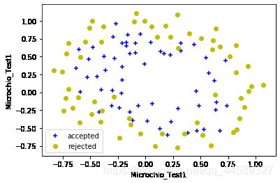
2正则化逻辑回归
filepath1=r'F:\jypternotebook\吴恩达机器学习python作业代码\code\ex2-logistic regression\ex2data2.txt'
ex2_data2=pd.read_csv(filepath1,header=None,names=['Microchio_Test1','Microchio_Test2','accepted_or_not'])
ex2_data2
| Microchio_Test1 | Microchio_Test2 | accepted_or_not | |
|---|---|---|---|
| 0 | 0.051267 | 0.699560 | 1 |
| 1 | -0.092742 | 0.684940 | 1 |
| 2 | -0.213710 | 0.692250 | 1 |
| 3 | -0.375000 | 0.502190 | 1 |
| 4 | -0.513250 | 0.465640 | 1 |
| ... | ... | ... | ... |
| 113 | -0.720620 | 0.538740 | 0 |
| 114 | -0.593890 | 0.494880 | 0 |
| 115 | -0.484450 | 0.999270 | 0 |
| 116 | -0.006336 | 0.999270 | 0 |
| 117 | 0.632650 | -0.030612 | 0 |
118 rows × 3 columns
plt.figure(figsize=(16,8))
accepted=ex2_data2[ex2_data2['accepted_or_not'].isin([1])]
rejected=ex2_data2[ex2_data2['accepted_or_not'].isin([0])]
plt.scatter(accepted['Microchio_Test1'],accepted['Microchio_Test2'],c='b',marker='+',label='accepted')
plt.scatter(rejected['Microchio_Test1'],rejected['Microchio_Test2'],c='y',marker='o',label='rejected')
plt.xlabel('Microchio_Test1')
plt.ylabel('Microchio_Test1')
plt.legend()
plt.show()
2.1MapFeature
#ex2_data2=data.insert(0,'ones',1)
mapFeature=pd.DataFrame([])
x1=np.array(ex2_data2['Microchio_Test1'])
x2=np.array(ex2_data2['Microchio_Test1'])
mapFeature['x1']=x1
mapFeature['x2']=x2
mapFeature.insert(0,'ones',1)
for i in range(2,7):
    for j in range(0,i+1):
        mapFeature['x1^'+str(i-j)+'x2^'+str(j)]=np.power(x1,i-j)*np.power(x2,j)
mapFeature
| ones | x1 | x2 | x1^2x2^0 | x1^1x2^1 | x1^0x2^2 | x1^3x2^0 | x1^2x2^1 | x1^1x2^2 | x1^0x2^3 | ... | x1^2x2^3 | x1^1x2^4 | x1^0x2^5 | x1^6x2^0 | x1^5x2^1 | x1^4x2^2 | x1^3x2^3 | x1^2x2^4 | x1^1x2^5 | x1^0x2^6 | |
|---|---|---|---|---|---|---|---|---|---|---|---|---|---|---|---|---|---|---|---|---|---|
| 0 | 1 | 0.051267 | 0.051267 | 0.002628 | 0.002628 | 0.002628 | 1.347453e-04 | 1.347453e-04 | 1.347453e-04 | 1.347453e-04 | ... | 3.541519e-07 | 3.541519e-07 | 3.541519e-07 | 1.815630e-08 | 1.815630e-08 | 1.815630e-08 | 1.815630e-08 | 1.815630e-08 | 1.815630e-08 | 1.815630e-08 |
| 1 | 1 | -0.092742 | -0.092742 | 0.008601 | 0.008601 | 0.008601 | -7.976812e-04 | -7.976812e-04 | -7.976812e-04 | -7.976812e-04 | ... | -6.860919e-06 | -6.860919e-06 | -6.860919e-06 | 6.362953e-07 | 6.362953e-07 | 6.362953e-07 | 6.362953e-07 | 6.362953e-07 | 6.362953e-07 | 6.362953e-07 |
| 2 | 1 | -0.213710 | -0.213710 | 0.045672 | 0.045672 | 0.045672 | -9.760555e-03 | -9.760555e-03 | -9.760555e-03 | -9.760555e-03 | ... | -4.457837e-04 | -4.457837e-04 | -4.457837e-04 | 9.526844e-05 | 9.526844e-05 | 9.526844e-05 | 9.526844e-05 | 9.526844e-05 | 9.526844e-05 | 9.526844e-05 |
| 3 | 1 | -0.375000 | -0.375000 | 0.140625 | 0.140625 | 0.140625 | -5.273438e-02 | -5.273438e-02 | -5.273438e-02 | -5.273438e-02 | ... | -7.415771e-03 | -7.415771e-03 | -7.415771e-03 | 2.780914e-03 | 2.780914e-03 | 2.780914e-03 | 2.780914e-03 | 2.780914e-03 | 2.780914e-03 | 2.780914e-03 |
| 4 | 1 | -0.513250 | -0.513250 | 0.263426 | 0.263426 | 0.263426 | -1.352032e-01 | -1.352032e-01 | -1.352032e-01 | -1.352032e-01 | ... | -3.561597e-02 | -3.561597e-02 | -3.561597e-02 | 1.827990e-02 | 1.827990e-02 | 1.827990e-02 | 1.827990e-02 | 1.827990e-02 | 1.827990e-02 | 1.827990e-02 |
| ... | ... | ... | ... | ... | ... | ... | ... | ... | ... | ... | ... | ... | ... | ... | ... | ... | ... | ... | ... | ... | ... |
| 113 | 1 | -0.720620 | -0.720620 | 0.519293 | 0.519293 | 0.519293 | -3.742131e-01 | -3.742131e-01 | -3.742131e-01 | -3.742131e-01 | ... | -1.943263e-01 | -1.943263e-01 | -1.943263e-01 | 1.400354e-01 | 1.400354e-01 | 1.400354e-01 | 1.400354e-01 | 1.400354e-01 | 1.400354e-01 | 1.400354e-01 |
| 114 | 1 | -0.593890 | -0.593890 | 0.352705 | 0.352705 | 0.352705 | -2.094682e-01 | -2.094682e-01 | -2.094682e-01 | -2.094682e-01 | ... | -7.388054e-02 | -7.388054e-02 | -7.388054e-02 | 4.387691e-02 | 4.387691e-02 | 4.387691e-02 | 4.387691e-02 | 4.387691e-02 | 4.387691e-02 | 4.387691e-02 |
| 115 | 1 | -0.484450 | -0.484450 | 0.234692 | 0.234692 | 0.234692 | -1.136964e-01 | -1.136964e-01 | -1.136964e-01 | -1.136964e-01 | ... | -2.668362e-02 | -2.668362e-02 | -2.668362e-02 | 1.292688e-02 | 1.292688e-02 | 1.292688e-02 | 1.292688e-02 | 1.292688e-02 | 1.292688e-02 | 1.292688e-02 |
| 116 | 1 | -0.006336 | -0.006336 | 0.000040 | 0.000040 | 0.000040 | -2.544062e-07 | -2.544062e-07 | -2.544062e-07 | -2.544062e-07 | ... | -1.021440e-11 | -1.021440e-11 | -1.021440e-11 | 6.472253e-14 | 6.472253e-14 | 6.472253e-14 | 6.472253e-14 | 6.472253e-14 | 6.472253e-14 | 6.472253e-14 |
| 117 | 1 | 0.632650 | 0.632650 | 0.400246 | 0.400246 | 0.400246 | 2.532156e-01 | 2.532156e-01 | 2.532156e-01 | 2.532156e-01 | ... | 1.013486e-01 | 1.013486e-01 | 1.013486e-01 | 6.411816e-02 | 6.411816e-02 | 6.411816e-02 | 6.411816e-02 | 6.411816e-02 | 6.411816e-02 | 6.411816e-02 |
118 rows × 28 columns
2.2 代价函数与梯度下降
regularized cost(正则化代价函数)
J ( θ ) = 1 m ∑ i = 1 m [ − y ( i ) log ( h θ ( x ( i ) ) ) − ( 1 − y ( i ) ) log ( 1 − h θ ( x ( i ) ) ) ] + λ 2 m ∑ j = 1 n θ j 2 J\left( \theta \right)=\frac{1}{m}\sum\limits_{i=1}^{m}{[-{{y}^{(i)}}\log \left( {{h}_{\theta }}\left( {{x}^{(i)}} \right) \right)-\left( 1-{{y}^{(i)}} \right)\log \left( 1-{{h}_{\theta }}\left( {{x}^{(i)}} \right) \right)]}+\frac{\lambda }{2m}\sum\limits_{j=1}^{n}{\theta _{j}^{2}} J(θ)=m1i=1∑m[−y(i)log(hθ(x(i)))−(1−y(i))log(1−hθ(x(i)))]+2mλj=1∑nθj2
def costreg(theta,X,Y,learningrate):
    X=np.array(X)
    m,n=X.shape
    Y=np.array(Y)
    error=sigmod(X.dot(theta))-Y
    first=-Y*np.log(sigmod(X.dot(theta)))
    second=-(1-Y)*np.log(1-sigmod(X.dot(theta)))
    J=np.sum(first+second)/m+(learningrate/(2*m))*np.sum(theta[1:]**2)
    return J
如果我们要使用梯度下降法令这个代价函数最小化,因为我们未对 θ 0 {{\theta }_{0}} θ0 进行正则化,所以梯度下降算法将分两种情形:
\begin{align}
& Repeat\text{ }until\text{ }convergence\text{ }!!{!!\text{ } \
& \text{ }{{\theta }{0}}:={{\theta }{0}}-a\frac{1}{m}\sum\limits_{i=1}^{m}{[{{h}{\theta }}\left( {{x}^{(i)}} \right)-{{y}{(i)}}]x_{_{0}}{(i)}} \
& \text{ }{{\theta }{j}}:={{\theta }{j}}-a\frac{1}{m}\sum\limits{i=1}^{m}{[{{h}{\theta }}\left( {{x}^{(i)}} \right)-{{y}{(i)}}]x_{j}{(i)}}+\frac{\lambda }{m}{{\theta }{j}} \
& \text{ }!!}!!\text{ } \
& Repeat \
\end{align}
对上面的算法中 j=1,2,…,n 时的更新式子进行调整可得:
θ j : = θ j ( 1 − a λ m ) − a 1 m ∑ i = 1 m ( h θ ( x ( i ) ) − y ( i ) ) x j ( i ) {{\theta }_{j}}:={{\theta }_{j}}(1-a\frac{\lambda }{m})-a\frac{1}{m}\sum\limits_{i=1}^{m}{({{h}_{\theta }}\left( {{x}^{(i)}} \right)-{{y}^{(i)}})x_{j}^{(i)}} θj:=θj(1−amλ)−am1i=1∑m(hθ(x(i))−y(i))xj(i)
def gradientReg(theta, X, Y, learningRate):
    X=np.array(X)
    m,n=X.shape
    Y=np.array(Y)
    grad=np.array(theta)
    error=sigmod(X.dot(theta))-Y
    for i in range(theta.size):
        if i==0:
            grad[i]=np.sum(error*X[:,i])/m
        else:
            grad[i]=np.sum(error*X[:,i])/m+(learningRate/m)*theta[i]
    return grad
lambda1=1
X2=np.array(mapFeature)
Y2=np.array(ex2_data2['accepted_or_not'])
theta=np.zeros(X2.shape[1])
costreg(theta, X2, Y2, lambda1)
0.6931471805599454
gradientReg(theta, X2, Y2, lambda1)
array([0.00847458, 0.01878809, 0.01878809, 0.05034464, 0.05034464,
       0.05034464, 0.01835599, 0.01835599, 0.01835599, 0.01835599,
       0.03934862, 0.03934862, 0.03934862, 0.03934862, 0.03934862,
       0.01997075, 0.01997075, 0.01997075, 0.01997075, 0.01997075,
       0.01997075, 0.03103124, 0.03103124, 0.03103124, 0.03103124,
       0.03103124, 0.03103124, 0.03103124])
import scipy.optimize as opt
result2 = opt.fmin_tnc(func=costreg, x0=theta, fprime=gradientReg, args=(X2, Y2, lambda1))
result2
(array([ 0.61880644,  0.02107357,  0.02107357, -0.47791542, -0.47791542,
        -0.47791542,  0.23492931,  0.23492931,  0.23492931,  0.23492931,
        -0.45461112, -0.45461111, -0.45461112, -0.45461111, -0.45461112,
         0.00540852,  0.00540852,  0.00540852,  0.00540852,  0.00540852,
         0.00540852, -0.36669469, -0.36669469, -0.36669469, -0.3666947 ,
        -0.36669469, -0.36669469, -0.36669469]), 27, 1)
theta_result=result2[0]
theta_result
array([ 0.55594786,  0.06259975,  0.06259975, -0.45266467, -0.45266467,
       -0.45266467,  0.12516208,  0.12516208,  0.12516208,  0.12516208,
       -0.36685169, -0.36685169, -0.36685169, -0.36685169, -0.36685169,
       -0.01262451, -0.01262451, -0.01262451, -0.01262451, -0.01262451,
       -0.01262451, -0.27394799, -0.27394799, -0.27394799, -0.27394799,
       -0.27394799, -0.27394799, -0.27394799])
predict2=predict(theta_result,X2)
accuracy2=(np.sum(predict2==Y2))/Y2.size
accuracy2
0.6779661016949152