基于python的音频信号处理
生成文件列表
采用递归方式读取指定目录下的文件列表
import os
def get_filelist(path, list):
    list_dir = os.listdir(path)
    for i in list_dir:
        sub_dir = os.path.join(path, i)
        if os.path.isdir(sub_dir):
            get_filelist(sub_dir, list)
        else:
            list.append(sub_dir)
读取wav文件
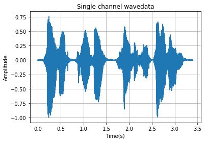
单通道 (matlab采用audioread实现)
读取音频的方式很多,主要要利用好数据量转换函数np.fromstring或np.frombuffer
import wave
import matplotlib.pyplot as plt
import numpy as np
import os

filepath = "./data/" #添加路径
filelist= os.listdir(filepath) #得到文件夹下的所有文件名称
f = wave.open(filepath+filelist[1],'rb')
params = f.getparams()
nchannels, sampwidth, framerate, nframes = params[:4]
strData = f.readframes(nframes)                  #读取音频,字符串格式
waveData = np.fromstring(strData,dtype=np.int16) #将字符串转化为int
waveData = waveData*1.0/(max(abs(waveData)))    #wave幅值归一化
# plot the wave
time = np.arange(0,nframes)*(1.0 / framerate)
plt.plot(time,waveData)
plt.xlabel("Time(s)")
plt.ylabel("Amplitude")
plt.title("Single channel wavedata")
plt.grid('on')#标尺,on:有,off:无。

##另一种语音读取方式
f = open(filepath+filelist[1],'rb')
bufferData = f.read()
waveData = np.frombuffer(bufferData, dtype=np.int16)
结果图:
多通道
这里通道数为3,主要借助np.reshape一下,其他同单通道处理完全一致
import wave
import matplotlib.pyplot as plt
import numpy as np
import os

filepath = "./data/" #添加路径
filelist= os.listdir(filepath) #得到文件夹下的所有文件名称
f = wave.open(filepath+filelist[0],'rb')
params = f.getparams()
nchannels, sampwidth, framerate, nframes = params[:4]
strData = f.readframes(nframes)                 #读取音频,字符串格式
waveData = np.fromstring(strData,dtype=np.int16)#将字符串转化为int
waveData = waveData*1.0/(max(abs(waveData)))   #wave幅值归一化
waveData = np.reshape(waveData,[nframes,nchannels])
f.close()
# plot the wave
time = np.arange(0,nframes)*(1.0 / framerate)
plt.figure()
plt.subplot(5,1,1)
plt.plot(time,waveData[:,0])
plt.xlabel("Time(s)")
plt.ylabel("Amplitude")
plt.title("Ch-1 wavedata")
plt.grid('on')#标尺,on:有,off:无。
plt.subplot(5,1,3)
plt.plot(time,waveData[:,1])
plt.xlabel("Time(s)")
plt.ylabel("Amplitude")
plt.title("Ch-2 wavedata")
plt.grid('on')#标尺,on:有,off:无。
plt.subplot(5,1,5)
plt.plot(time,waveData[:,2])
plt.xlabel("Time(s)")
plt.ylabel("Amplitude")
plt.title("Ch-3 wavedata")
plt.grid('on')#标尺,on:有,off:无。
plt.show()
效果图:
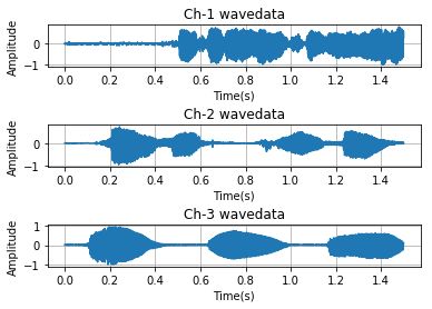
单通道为多通道的特例,所以多通道的读取方式对任意通道wav文件都适用。需要注意的是,waveData在reshape之后,与之前的数据结构是不同的。即waveData[0]等价于reshape之前的waveData,但不影响绘图分析,只是在分析频谱时才有必要考虑这一点。
写入wav文件
matlab采用audiowrite实现
单通道数据写入:
import wave
#import matplotlib.pyplot as plt
import numpy as np
import os
import struct

#wav文件读取
filepath = "./data/" #添加路径
filenlist= os.listdir(filepath) #得到文件夹下的所有文件名称
f = wave.open(filepath+filelist[1],'rb')
params = f.getparams()
nchannels, sampwidth, framerate, nframes = params[:4]
strData = f.readframes(nframes)#读取音频,字符串格式
waveData = np.fromstring(strData,dtype=np.int16)#将字符串转化为int
waveData = waveData*1.0/(max(abs(waveData)))#wave幅值归一化
f.close()
#wav文件写入
outData = waveData#待写入wav的数据,这里仍然取waveData数据
outfile = filepath+'out1.wav'
outwave = wave.open(outfile, 'wb')#定义存储路径以及文件名
nchannels = 1
sampwidth = 2
fs = 8000
data_size = len(outData)
framerate = int(fs)
nframes = data_size
comptype = "NONE"
compname = "not compressed"
outwave.setparams((nchannels, sampwidth, framerate, nframes,
    comptype, compname))

for v in outData:
    outwave.writeframes(struct.pack('h', int(v * 64000 / 2)))#outData:16位,-32767~32767,注意不要溢出
outwave.close()多通道数据写入:
多通道的写入与多通道读取类似,多通道读取是将一维数据reshape为二维,多通道的写入是将二维的数据reshape为一维,其实就是一个逆向的过程:
import wave
#import matplotlib.pyplot as plt
import numpy as np
import os
import struct

#wav文件读取
filepath = "./data/" #添加路径
filelist= os.listdir(filepath) #得到文件夹下的所有文件名称
f = wave.open(filepath+filelist[0],'rb')
params = f.getparams()
nchannels, sampwidth, framerate, nframes = params[:4]
strData = f.readframes(nframes)#读取音频,字符串格式
waveData = np.fromstring(strData,dtype=np.int16)#将字符串转化为int
waveData = waveData*1.0/(max(abs(waveData)))#wave幅值归一化
waveData = np.reshape(waveData,[nframes,nchannels])
f.close()
#wav文件写入
outData = waveData#待写入wav的数据,这里仍然取waveData数据
outData = np.reshape(outData,[nframes*nchannels,1])
outfile = filepath+'out2.wav'
outwave = wave.open(outfile, 'wb')#定义存储路径以及文件名
nchannels = 3
sampwidth = 2
fs = 8000
data_size = len(outData)
framerate = int(fs)
nframes = data_size
comptype = "NONE"
compname = "not compressed"
outwave.setparams((nchannels, sampwidth, framerate, nframes,
    comptype, compname))

for v in outData:
    outwave.writeframes(struct.pack('h', int(v * 64000 / 2)))#outData:16位,-32767~32767,注意不要溢出
outwave.close()
信号加窗
通常对信号截断、分帧需要加窗,因为截断都有频域能量泄露,而窗函数可以减少截断带来的影响。
窗函数在scipy.signal信号处理工具箱中,如hamming窗:
import pylab as pl
import scipy.signal as signal
pl.figure(figsize=(6,2))
pl.plot(signal.hanning(512))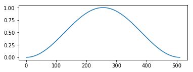
信号分帧
信号分帧的理论依据,其中x是语音信号,w是窗函数:
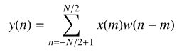
加窗截断类似采样,为了保证相邻帧不至于差别过大,通常帧与帧之间有帧移,其实就是插值平滑的作用。
给出示意图:

这是没有加窗的示例:
import numpy as np
import wave
import os
#import math

def enframe(signal, nw, inc):
    '''将音频信号转化为帧。
    参数含义:
    signal:原始音频型号
    nw:每一帧的长度(这里指采样点的长度,即采样频率乘以时间间隔)
    inc:相邻帧的间隔(同上定义)
    '''
    signal_length=len(signal) #信号总长度
    if signal_length<=nw: #若信号长度小于一个帧的长度,则帧数定义为1
        nf=1
    else: #否则,计算帧的总长度
        nf=int(np.ceil((1.0*signal_length-nw+inc)/inc))
    pad_length=int((nf-1)*inc+nw) #所有帧加起来总的铺平后的长度
    zeros=np.zeros((pad_length-signal_length,)) #不够的长度使用0填补,类似于FFT中的扩充数组操作
    pad_signal=np.concatenate((signal,zeros)) #填补后的信号记为pad_signal
    indices=np.tile(np.arange(0,nw),(nf,1))+np.tile(np.arange(0,nf*inc,inc),(nw,1)).T  #相当于对所有帧的时间点进行抽取,得到nf*nw长度的矩阵
    indices=np.array(indices,dtype=np.int32) #将indices转化为矩阵
    frames=pad_signal[indices] #得到帧信号
#    win=np.tile(winfunc(nw),(nf,1))  #window窗函数,这里默认取1
#    return frames*win   #返回帧信号矩阵
    return frames
def wavread(filename):
    f = wave.open(filename,'rb')
    params = f.getparams()
    nchannels, sampwidth, framerate, nframes = params[:4]
    strData = f.readframes(nframes)#读取音频,字符串格式
    waveData = np.fromstring(strData,dtype=np.int16)#将字符串转化为int
    f.close()
    waveData = waveData*1.0/(max(abs(waveData)))#wave幅值归一化
    waveData = np.reshape(waveData,[nframes,nchannels]).T
    return waveData

filepath = "./data/" #添加路径
dirname= os.listdir(filepath) #得到文件夹下的所有文件名称
filename = filepath+dirname[0]
data = wavread(filename)
nw = 512
inc = 128
Frame = enframe(data[0], nw, inc)
如果需要加窗,只需要将函数修改为:
def enframe(signal, nw, inc, winfunc):
    '''将音频信号转化为帧。
    参数含义:
    signal:原始音频型号
    nw:每一帧的长度(这里指采样点的长度,即采样频率乘以时间间隔)
    inc:相邻帧的间隔(同上定义)
    '''
    signal_length=len(signal) #信号总长度
    if signal_length<=nw: #若信号长度小于一个帧的长度,则帧数定义为1
        nf=1
    else: #否则,计算帧的总长度
        nf=int(np.ceil((1.0*signal_length-nw+inc)/inc))
    pad_length=int((nf-1)*inc+nw) #所有帧加起来总的铺平后的长度
    zeros=np.zeros((pad_length-signal_length,)) #不够的长度使用0填补,类似于FFT中的扩充数组操作
    pad_signal=np.concatenate((signal,zeros)) #填补后的信号记为pad_signal
    indices=np.tile(np.arange(0,nw),(nf,1))+np.tile(np.arange(0,nf*inc,inc),(nw,1)).T  #相当于对所有帧的时间点进行抽取,得到nf*nw长度的矩阵
    indices=np.array(indices,dtype=np.int32) #将indices转化为矩阵
    frames=pad_signal[indices] #得到帧信号
    win=np.tile(winfunc,(nf,1))  #window窗函数,这里默认取1
    return frames*win   #返回帧信号矩阵
其中窗函数,以hamming窗为例:
winfunc = signal.hamming(nw)
Frame = enframe(data[0], nw, inc, winfunc)
调用即可。
语谱图
其实得到了分帧信号,频域变换取幅值,就可以得到语谱图,如果仅仅是观察,matplotlib.pyplot有specgram指令:
import wave
import matplotlib.pyplot as plt
import numpy as np
import os

filepath = "./data/" #添加路径
filename= os.listdir(filepath) #得到文件夹下的所有文件名称
f = wave.open(filepath+filename[0],'rb')
params = f.getparams()
nchannels, sampwidth, framerate, nframes = params[:4]
strData = f.readframes(nframes)#读取音频,字符串格式
waveData = np.fromstring(strData,dtype=np.int16)#将字符串转化为int
waveData = waveData*1.0/(max(abs(waveData)))#wave幅值归一化
waveData = np.reshape(waveData,[nframes,nchannels]).T
f.close()
# plot the wave
plt.specgram(waveData[0],Fs = framerate, scale_by_freq = True, sides = 'default')
plt.ylabel('Frequency(Hz)')
plt.xlabel('Time(s)')
plt.show()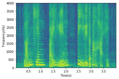
STFT和iSTFT
def stft(signal, window, win_size, hop_size, last_sample=False):
    """Convert time-domain signal to time-frequency domain.

    Args:
        signal   : multi-channel time-domain signal
        window   : window function, see cola_hamming as an example.
        win_size : window size (number of samples)
        hop_size : hop size (number of samples)
        last_sample : include last sample, by default (due to legacy bug),
                      the last sample is not included.

    Returns:
        tf       : multi-channel time-frequency domain signal.
    """
    assert signal.ndim == 2
    w = window(win_size, hop_size)
    return np.array([[
        np.fft.fft(c[t:t + win_size] * w)
        for t in range(0,
                       len(c) - win_size + (1 if last_sample else 0), hop_size)
    ] for c in signal])


def istft(tf, hop_size):
    """Inverse STFT

    Args:
        tf       : multi-channel time-frequency domain signal.
        hop_size : hop size (number of samples)

    Returns:
        signal   : multi-channel time-domain signal
    """
    tf = np.asarray(tf)
    nch, nframe, nfbin = tf.shape
    signal = np.zeros((nch, (nframe - 1) * hop_size + nfbin))
    for t in range(nframe):
        signal[:, t*hop_size:t*hop_size+nfbin] += \
                np.real(np.fft.ifft(tf[:, t]))
    return signal
计算导向矢量
def steering_vector(delay, win_size=0, fbins=None, fs=None):
    """Compute the steering vector.

    One and only one of the conditions are true:
        - win_size != 0
        - fbins is not None

    Args:
        delay : delay of each channel (see compute_delay),
                unit is second if fs is not None, otherwise sample
        win_size : (default 0) window (FFT) size. If zero, use fbins.
        fbins : (default None) center of frequency bins, as discrete value.
        fs    : (default None) sample rate


    Returns:
        stv   : steering vector, indices (cf)
    """
    assert (win_size != 0) != (fbins is not None)
    delay = np.asarray(delay)
    if fs is not None:
        delay *= fs  # to discrete-time value
    if fbins is None:
        fbins = np.fft.fftfreq(win_size)
    return np.exp(-2j * math.pi * np.outer(delay, fbins))
计算延时
def compute_delay(m_pos, doa, c=340, fs=None):
    """Compute delay of signal arrival at microphones.

    Args:
        m_pos : microphone positions, (M,3) array,
                M is number of microphones.
        doa   : direction of arrival, (3,) array or (N,3) array,
                N is the number of sources.
        c     : (default 340) speed of sound (m/s).
        fs    : (default None) sample rate.

    Return:
        delay : delay with reference of arrival at first microphone.
                first element is always 0.
                unit is second if fs is None, otherwise sample.
    """
    m_pos = np.asarray(m_pos)
    doa = np.asarray(doa)

    # relative position wrt first microphone
    r_pos = m_pos - m_pos[0]

    # inner product -> different in time
    if doa.ndim == 1:
        doa /= np.sqrt(np.sum(doa**2.0))  # normalize
        diff = -np.einsum('ij,j->i', r_pos, doa) / c
    else:
        assert doa.ndim == 2
        doa /= np.sqrt(np.sum(doa**2.0, axis=1, keepdims=True))  # normalize
        diff = -np.einsum('ij,kj->ki', r_pos, doa) / c

    if fs is not None:
        return diff * fs
    else:
        return diff
计算协方差矩阵
def cov_matrix(tf):
    """Covariance matrix of the  multi-channel signal.

    Args:
        tf  : multi-channel time-frequency domain signal.

    Returns:
        cov : covariance matrix, indexed by (ccf)
    """
    nch, nframe, nfbin = tf.shape
    return np.einsum('itf,jtf->ijf', tf, tf.conj()) / float(nframe)
11. VAD操作
def vad_by_threshold(fs, sig, vadrate, threshold_db, neighbor_size=0):
    """Voice Activity Detection by threshold

    Args:
        fs       : sample rate.
        signal   : multi-channel time-domain signal.
        vadrate  : output vad rate
        threshold_db : threshold in decibel
        neighbor_size : half size of (excluding center) neighbor area

    Returns:
        vad      : VAD label (0: silence, 1: active)
    """
    nch, nsamples = sig.shape
    nframes = nsamples * vadrate / fs
    fpower = np.zeros((nch, nframes))  # power at frame level
    for i in range(nframes):
        fpower[:, i] = power(sig[:,
                                 (i * fs / vadrate):((i + 1) * fs / vadrate)])

    # average power in neighbor area
    if neighbor_size == 0:
        apower = fpower
    else:
        apower = np.zeros((nch, nframes))
        for i in range(nframes):
            apower[:, i] = np.mean(
                fpower[:,
                       max(0, i - neighbor_size):min(nframes, i +
                                                     neighbor_size + 1)],
                axis=1)
    return (apower > 10.0**(threshold_db / 10.0)).astype(int)
参考资料
https://www.cnblogs.com/xingshansi/p/6799994.html
https://lxp-never.blog.csdn.net/article/details/84967662
https://github.com/hwp/apkit