LESSON 9.4 集成算法的参数空间与网格优化

四 集成算法的参数空间与网格优化

如随机森林中所展示的，集成算法的超参数种类繁多、取值丰富，且参数之间会相互影响、共同作用于算法的最终结果，因此集成算法的调参是一个难度很高的过程。在超参数优化还未盛行的时候，随机森林的调参是基于方差-偏差理论（variance-bias trade-off）和学习曲线完成的，而现在我们可以依赖于网格搜索来完成自动优化。在对任意算法进行网格搜索时，我们需要明确两个基本事实

1、参数对算法结果的影响力大小
2、用于进行搜索的参数空间

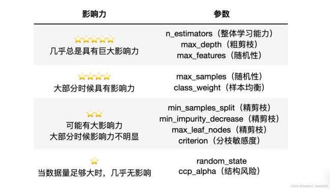
对随机森林来说，我们可以大致如下排列各个参数对算法的影响：

随机森林在剪枝方面的空间总是很大的，因为默认参数下树的结构基本没有被影响（也就是几乎没有剪枝），因此当随机森林过拟合的时候，我们可以尝试粗、精、随机等各种方式来影响随机森林。通常在网格搜索当中，我们会考虑所有有巨大影响力的参数、以及1、2个影响力不明显的参数。

虽然随机森林调参的空间较大，大部分人在调参过程中依然难以突破，因为树的集成模型的参数空间非常难以确定。当没有数据支撑时，人们很难通过感觉或经验来找到正确的参数范围。举例来说，我们也很难直接判断究竟多少棵树对于当前的模型最有效，同时，我们也很难判断不剪枝时一棵决策树究竟有多深、有多少叶子、或者一片叶子上究竟有多少个样本，更不要谈凭经验判断树模型整体的不纯度情况了。可以说，当森林建好之后，我们简直是对森林一无所知。对于网格搜索来说，新增一个潜在的参数可选值，计算量就会指数级增长，因此找到有效的参数空间非常重要。此时我们就要引入两个工具来帮助我们：

1、学习曲线
2、决策树对象Tree的属性

• 学习曲线

学习曲线是以参数的不同取值为横坐标，模型的结果为纵坐标的曲线。当模型的参数较少、且参数之间的相互作用较小时，我们可以直接使用学习曲线进行调参。但对于集成算法来说，学习曲线更多是我们探索参数与模型关系的关键手段。许多参数对模型的影响是确定且单调的，例如`n_estimators`，树越多模型的学习能力越强，再比如`ccp_alpha`，该参数值越大模型抗过拟合能力越强，因此我们可能通过学习曲线找到这些参数对模型影响的极限。我们会围绕这些极限点来构筑我们的参数空间。

先来看看n_estimators的学习曲线：

#参数潜在取值，由于现在我们只调整一个参数，因此参数的范围可以取大一些、取值也可以更密集
Option = [1,*range(5,101,5)]

#生成保存模型结果的arrays
trainRMSE = np.array([])
testRMSE = np.array([])
trainSTD = np.array([])
testSTD = np.array([])

#在参数取值中进行循环
for n_estimators in Option:
    
    #按照当下的参数，实例化模型
    reg_f = RFR(n_estimators=n_estimators,random_state=1412)
    
    #实例化交叉验证方式，输出交叉验证结果
    cv = KFold(n_splits=5,shuffle=True,random_state=1412)
    result_f = cross_validate(reg_f,X,y,cv=cv,scoring="neg_mean_squared_error"
                              ,return_train_score=True
                              ,n_jobs=-1)
    
    #根据输出的MSE进行RMSE计算
    train = abs(result_f["train_score"])**0.5
    test = abs(result_f["test_score"])**0.5
    
    #将本次交叉验证中RMSE的均值、标准差添加到arrays中进行保存
    trainRMSE = np.append(trainRMSE,train.mean()) #效果越好
    testRMSE = np.append(testRMSE,test.mean())
    trainSTD = np.append(trainSTD,train.std()) #模型越稳定
    testSTD = np.append(testSTD,test.std())

def plotCVresult(Option,trainRMSE,testRMSE,trainSTD,testSTD):
    #一次交叉验证下，RMSE的均值与std的绘图
    xaxis = Option
    plt.figure(figsize=(8,6),dpi=80)

    #RMSE
    plt.plot(xaxis,trainRMSE,color="k",label = "RandomForestTrain")
    plt.plot(xaxis,testRMSE,color="red",label = "RandomForestTest")

    #标准差 - 围绕在RMSE旁形成一个区间
    plt.plot(xaxis,trainRMSE+trainSTD,color="k",linestyle="dotted")
    plt.plot(xaxis,trainRMSE-trainSTD,color="k",linestyle="dotted")
    plt.plot(xaxis,testRMSE+testSTD,color="red",linestyle="dotted")
    plt.plot(xaxis,testRMSE-testSTD,color="red",linestyle="dotted")
    plt.xticks([*xaxis])
    plt.legend(loc=1)
    plt.show()

plotCVresult(Option,trainRMSE,testRMSE,trainSTD,testSTD)

当绘制学习曲线时，我们可以很容易找到泛化误差开始上升、或转变为平稳趋势的转折点。因此我们可以选择转折点或转折点附近的n_estimators取值，例如20。然而，n_estimators会受到其他参数的影响，例如：

• 单棵决策树的结构更简单时（依赖剪枝时），可能需要更多的树
• 单棵决策树训练的数据更简单时（依赖随机性时），可能需要更多的树

因此n_estimators的参数空间可以被确定为range(20,100,5)，如果你比较保守，甚至可以确认为是range(15,25,5)。

• 决策树对象Tree

在sklearn中，树模型是单独的一类对象，每个树模型背后都有一套完整的属性供我们调用，包括树的结构、树的规模等众多细节。在之前的课程中，我们曾经使用过树模型的绘图功能plot_tree，除此之外树还有许多有用的属性。随机森林是树组成的算法，因此也可以调用这些属性。我们来举例说明：

reg_f = RFR(n_estimators=10,random_state=1412)
reg_f = reg_f.fit(X,y) #训练一个随机森林

属性.estimators_，查看森林中所有的树

reg_f.estimators_ #一片随机森林中所有的树
# [DecisionTreeRegressor(max_features='auto', random_state=1630984966),
#  DecisionTreeRegressor(max_features='auto', random_state=472863509),
#  DecisionTreeRegressor(max_features='auto', random_state=1082704530),
#  DecisionTreeRegressor(max_features='auto', random_state=1930362544),
#  DecisionTreeRegressor(max_features='auto', random_state=273973624),
#  DecisionTreeRegressor(max_features='auto', random_state=21991934),
#  DecisionTreeRegressor(max_features='auto', random_state=1886585710),
#  DecisionTreeRegressor(max_features='auto', random_state=63725675),
#  DecisionTreeRegressor(max_features='auto', random_state=1374343434),
#  DecisionTreeRegressor(max_features='auto', random_state=1078007175)]

#可以用索引单独提取一棵树
reg_f.estimators_[0]
#DecisionTreeRegressor(max_features='auto', random_state=1630984966)

#调用这棵树的底层结构
reg_f.estimators_[0].tree_
#

属性.max_depth，查看当前树的实际深度

reg_f.estimators_[0].tree_.max_depth #max_depth=None
#19

#对森林中所有树查看实际深度
for t in reg_f.estimators_:
    print(t.tree_.max_depth)
#19
#25
#27
#20
#23
#22
#22
#20
#22
#24

#如果树的数量较多，也可以查看平均或分布
reg_f = RFR(n_estimators=100,random_state=1412)
reg_f = reg_f.fit(X,y) #训练一个随机森林
d = pd.Series([],dtype="int64")
for idx,t in enumerate(reg_f.estimators_):
    d[idx] = t.tree_.max_depth

d.mean()
#22.25

d.describe()
#count    100.000000
#mean      22.250000
#std        1.955954
#min       19.000000
#25%       21.000000
#50%       22.000000
#75%       23.000000
#max       30.000000
#dtype: float64

假设现在你的随机森林过拟合，max_depth的最大深度范围设置在[15,25]之间就会比较有效，如果我们希望激烈地剪枝，则可以设置在[10,15]之间。

相似的，我们也可以调用其他属性来辅助我们调参：

#一棵树上的总叶子量
reg_f.estimators_[0].tree_.node_count
#1807

#所有树上的总叶子量
for t in reg_f.estimators_:
    print(t.tree_.node_count)
#1807
#1777
#1763
#1821
#1777
#1781
#1811
#1771
#1753
#1779

 根据经验，当决策树不减枝且在训练集上的预测结果不错时，一棵树上的叶子量常常与样本量相当或比样本量更多，算法结果越糟糕，叶子量越少，如果RMSE很高或者R2很低，则可以考虑使用样本量的一半或3/4作为不减枝时的叶子量的参考。

#每个节点上的不纯度下降量，为-2则表示该节点是叶子节点
reg_f.estimators_[0].tree_.threshold.tolist()[:20]
# [6.5,
#  5.5,
#  327.0,
#  214.0,
#  0.5,
#  1.0,
#  104.0,
#  0.5,
#  -2.0,
#  -2.0,
#  -2.0,
#  105.5,
#  28.5,
#  0.5,
#  1.5,
#  -2.0,
#  -2.0,
#  11.0,
#  1212.5,
#  2.5]

#你怎么知道min_impurity_decrease的范围设置多少会剪掉多少叶子？
pd.Series(reg_f.estimators_[0].tree_.threshold).value_counts().sort_index()
#-2.0       904
# 0.5        43
# 1.0        32
# 1.5        56
# 2.0        32
#          ... 
# 1118.5      1
# 1162.5      1
# 1212.5      2
# 1254.5      1
# 1335.5      1
#Length: 413, dtype: int64

pd.set_option("display.max_rows",None)
np.cumsum(pd.Series(reg_f.estimators_[0].tree_.threshold).value_counts().sort_index()[1:])
#1.0        32
#1.5        88
#2.0       120
#2.5       167
#...       ...
#1212.5    858
#1254.5    859
#1335.5    860
#dtype: int64

从这棵树反馈的结果来看，min_impurity_decrease在现在的数据集上至少要设置到[2,10]的范围才可能对模型有较大的影响。

#min_sample_split的范围要如何设置才会剪掉很多叶子？
np.bincount(reg_f.estimators_[0].tree_.n_node_samples.tolist())[:10]
#array([  0, 879, 321, 154,  86,  52,  42,  38,  29,  18], dtype=int64)

更多属性可以参考：

from sklearn.tree._tree import Tree
type(Tree)
#type
help(Tree)

• 使用网格搜索在随机森林上进行调参

现在模型正处于过拟合的状态，需要抗过拟合，且整体数据量不是非常多，随机抽样的比例不宜减小，因此我们挑选以下五个参数进行搜索：n_estimators，max_depth，max_features，min_impurity_decrease，criterion。

import numpy as np
import pandas as pd
import sklearn
import matplotlib as mlp
import matplotlib.pyplot as plt
import time #计时模块time
from sklearn.ensemble import RandomForestRegressor as RFR
from sklearn.model_selection import cross_validate, KFold, GridSearchCV

def RMSE(cvresult,key):
    return (abs(cvresult[key])**0.5).mean()

data = pd.read_csv(r"D:\Pythonwork\2021ML\PART 2 Ensembles\datasets\House Price\train_encode.csv",index_col=0)

X = data.iloc[:,:-1]
y = data.iloc[:,-1]
X.shape
#(1460, 80)

X.head()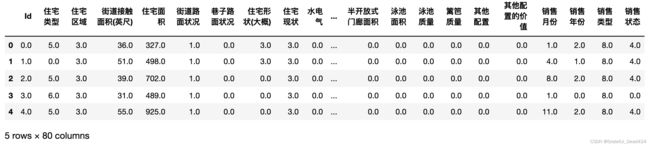

Step 1.建立benchmark 

reg = RFR(random_state=1412)
cv = KFold(n_splits=5,shuffle=True,random_state=1412)

result_pre_adjusted = cross_validate(reg,X,y,cv=cv,scoring="neg_mean_squared_error"
                          ,return_train_score=True
                          ,verbose=True
                          ,n_jobs=-1)

RMSE(result_pre_adjusted,"train_score")
#11177.272008319653

RMSE(result_pre_adjusted,"test_score")
#30571.26665524217

Step 2.创建参数空间

param_grid_simple = {"criterion": ["squared_error","poisson"]
                     , 'n_estimators': [*range(20,100,5)]
                     , 'max_depth': [*range(10,25,2)]
                     , "max_features": ["log2","sqrt",16,32,64,"auto"]
                     , "min_impurity_decrease": [*np.arange(0,5,10)]
                    }

Step 3.实例化用于搜索的评估器、交叉验证评估器与网格搜索评估器

#n_jobs=4/8,verbose=True
reg = RFR(random_state=1412,verbose=True,n_jobs=-1)
cv = KFold(n_splits=5,shuffle=True,random_state=1412)
search = GridSearchCV(estimator=reg
                     ,param_grid=param_grid_simple
                     ,scoring = "neg_mean_squared_error"
                     ,verbose = True
                     ,cv = cv
                     ,n_jobs=-1)

Step 4.训练网格搜索评估器

#=====【TIME WARNING: 7mins】=====#
start = time.time()
search.fit(X,y)
print(time.time() - start)
#Fitting 5 folds for each of 1536 candidates, totalling 7680 fits
#381.6039867401123

Step 5.查看结果

search.best_estimator_
#RandomForestRegressor(max_depth=23, max_features=16, min_impurity_decrease=0,
#                      n_estimators=85, n_jobs=-1, random_state=1412,
#                      verbose=True)

abs(search.best_score_)**0.5
#29179.698261599166

ad_reg = RFR(n_estimators=85, max_depth=23, max_features=16, random_state=1412)
cv = KFold(n_splits=5,shuffle=True,random_state=1412)
result_post_adjusted = cross_validate(ad_reg,X,y,cv=cv,scoring="neg_mean_squared_error"
                          ,return_train_score=True
                          ,verbose=True
                          ,n_jobs=-1)

RMSE(result_post_adjusted,"train_score")
#11000.81099038192

RMSE(result_post_adjusted,"test_score")
#28572.070208366855

#默认值下随机森林的RMSE
xaxis = range(1,6)
plt.figure(figsize=(8,6),dpi=80)
#RMSE
plt.plot(xaxis,abs(result_pre_adjusted["train_score"])**0.5,color="green",label = "RF_pre_ad_Train")
plt.plot(xaxis,abs(result_pre_adjusted["test_score"])**0.5,color="green",linestyle="--",label = "RF_pre_ad_Test")
plt.plot(xaxis,abs(result_post_adjusted["train_score"])**0.5,color="orange",label = "RF_post_ad_Train")
plt.plot(xaxis,abs(result_post_adjusted["test_score"])**0.5,color="orange",linestyle="--",label = "RF_post_ad_Test")
plt.xticks([1,2,3,4,5])
plt.xlabel("CVcounts",fontsize=16)
plt.ylabel("RMSE",fontsize=16)
plt.legend()
plt.show()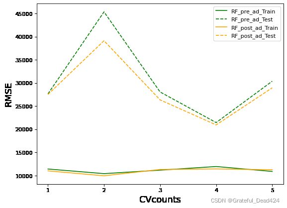

不难发现，网格搜索之后的模型过拟合程度减轻，且在训练集与测试集上的结果都有提高，可以说从根本上提升了模型的基础能力。我们还可以根据网格的结果继续尝试进行其他调整，来进一步降低模型在测试集上的RMSE。