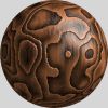
Perlin Noise

come from:http://freespace.virgin.net/hugo.elias/models/m_perlin.htm

Many people have used random number generators in their programs to create unpredictability, make the motion and behavior of objects appear more natural, or generate textures. Random number generators certainly have their uses, but at times their output can be too harsh to appear natural. This article will present a function which has a very wide range of uses, more than I can think of, but basically anywhere where you need something to look natural in origin. What's more it's output can easily be tailored to suit your needs.

 

If you look at many things in nature, you will notice that they are fractal. They have various levels of detail. A common example is the outline of a mountain range. It contains large variations in height (the mountains), medium variations (hills), small variations (boulders), tiny variations (stones) . . . you could go on. Look at almost anything: the distribution of patchy grass on a field, waves in the sea, the movements of an ant, the movement of branches of a tree, patterns in marble, winds. All these phenomena exhibit the same pattern of large and small variations. The Perlin Noise function recreates this by simply adding up noisy functions at a range of different scales.

 

To create a Perlin noise function, you will need two things, a Noise Function, and an Interpolation Function.

Introduction To Noise Functions

A noise function is essentially a seeded random number generator. It takes an integer as a parameter, and returns a random number based on that parameter. If you pass it the same parameter twice, it produces the same number twice. It is very important that it behaves in this way, otherwise the Perlin function will simply produce nonsense.

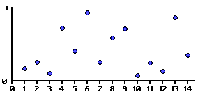
Here is a graph showing an example noise function. A random value between 0 and 1 is assigned to every point on the X axis.

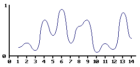
By smoothly interpolating between the values, we can define a continuous function that takes a non-integer as a parameter. I will discuss various ways of interpolating the values later in this article.

Definitions

Before I go any further, let me define what I mean by amplitude and frequency. If you have studied physics, you may well have come across the concept of amplitude and frequency applied to a sin wave.

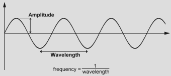	Sin Wave The wavelength of a sin wave is the distance from one peak to another. The amplitude is the height of the wave. The frequency is defined to be 1/wavelength.
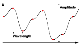	Noise Wave In the graph of this example noise function, the red spots indicate the random values defined along the dimension of the function. In this case, the amplitude is the difference between the minimum and maximum values the function could have. The wavelength is the distance from one red spot to the next. Again frequency is defined to be 1/wavelength.

Creating the Perlin Noise Function

Now, if you take lots of such smooth functions, with various frequencies and amplitudes, you can add them all together to create a nice noisy function. This is the Perlin Noise Function.

Take the following Noise Functions

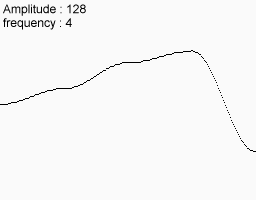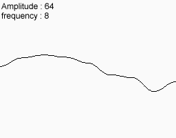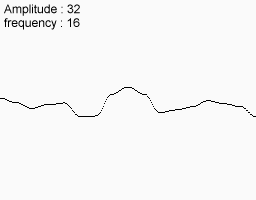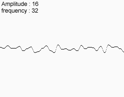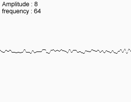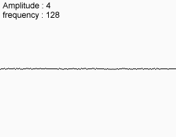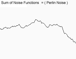
Add them together, and this is what you get.   You can see that this function has large, medium and small variations. You may even imagine that it looks a little like a mountain range. In fact many computer generated landscapes are made using this method. Of course they use 2D noise, which I shall get onto in a moment.

 

You can, of course, do the same in 2 dimensions.

Some noise functions are created in 2D

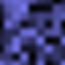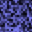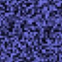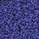Adding all these functions together produces a noisy pattern.

Persistence

When you're adding together these noise functions, you may wonder exactly what amplitude and frequency to use for each one. The one dimensional example above used twice the frequency and half the amplitude for each successive noise function added. This is quite common. So common in fact, that many people don't even consider using anything else. However, you can create Perlin Noise functions with different characteristics by using other frequencies and amplitudes at each step. For example, to create smooth rolling hills, you could use Perlin noise function with large amplitudes for the low frequencies , and very small amplitudes for the higher frequencies. Or you could make a flat, but very rocky plane choosing low amplitudes for low frequencies.

 

To make it simpler, and to avoid repeating the words Amplitude and Frequency all the time, a single number is used to specify the amplitude of each frequency. This value is known as Persistence. There is some ambiguity as to it's exact meaning. The term was originally coined by Mandelbrot, one of the people behind the discovery of fractals. He defined noise with a lot of high frequency as having a low persistence. My friend Matt also came up with the concept of persistence, but defined it the other way round. To be honest, I prefer Matt's definition. Sorry Mandelbrot. So our definition of persistence is this:

 

frequency = 2i

amplitude = persistencei

 

Where i is the i^th noise function being added. To illustrate the effect of persistence on the output of the Perlin Noise, take a look at the diagrams below. They show the component noise functions that are added, the effect of the persistence value, and the resultant Perlin noise function.

Frequency

1

2

4

8

16

32

Persistence = 1/4

+

+

+

+

+

=

Amplitude:

1

1/4

1/16

1/64

1/256

1/1024

result

Persistence = 1/2

+

+

+

+

+

=

Amplitude:

1

1/2

1/4

1/8

1/16

1/32

result

Persistence = 1 / root2

+

+

+

+

+

=

Amplitude:

1

1/1.414

1/2

1/2.828

1/4

1/5.656

result

Persistence = 1

+

+

+

+

+

=

Amplitude:

1

1

1

1

1

1

result

 

Octaves

Each successive noise function you add is known as an octave. The reason for this is that each noise function is twice the frequency of the previous one. In music, octaves also have this property.Exactly how many octaves you add together is entirely up to you. You may add as many or as few as you want. However, let me give you some suggestions. If you are using the perlin noise function to render an image to the screen, there will come a point when an octave has too high a frequency to be displayable. There simply may not be enough pixels on the screen to reproduce all the little details of a very high frequency noise function. Some implementations of Perlin Noise automatically add up as many noise functions they can until the limits of the screen (or other medium) are reached.It is also wise to stop adding noise functions when their amplitude becomes too small to reproduce. Exactly when that happens depends on the level of persistence, the overall amplitude of the Perlin function and the bit resolution of your screen (or whatever).

Making your noise functions

What do we look for in a noise function? Well, it's essentially a random number generator. However, unlike other random number generators you may have come across in your programs which give you a different random number every time you call them, these noise functions supply a random number calculated from one or more parameters. I.e. every time you pass the same number to the noise function, it will respond with the same number. But pass it a different number, and it will return a different number.

 

Well, I don't know a lot about random number generators, so I went looking for some, and here's one I found. It seems to be pretty good. It returns floating point numbers between -1.0 and 1.0.

function IntNoise(32-bit integer: x) x = (x<<13) ^ x; return ( 1.0 - ( (x * (x * x * 15731 + 789221) + 1376312589) & 7fffffff) / 1073741824.0); end IntNoise function

 

Now, you'll want several different random number generators, so I suggest making several copies of the above code, but use slightly different numbers. Those big scarey looking numbers are all prime numbers, so you could just use some other prime numbers of a similar size. So, to make it easy for you to find random numbers, I have written a little program to list prime numbers for you. You can give it a start number and an end number, and it will find all the primes between the two. Source code is also included, so you can easily include it into your own programs to produce a random prime number. Primes.zip

Interpolation

Having created your noise function, you will need to smooth out the values it returns. Again, you can choose any method you like, but some look better than others. A standard interpolation function takes three inputs, a and b, the values to be interpolated between, and x which takes a value between 0 and 1. The Interpolation function returns a value between a and b based on the value x. When x equals 0, it returns a, and when x is 1, it returns b. When x is between 0 and 1, it returns some value between a and b.

Linear Interpolation: Looks awful, like those cheap 'plasmas' that everyone uses to generate landscapes. It's a simple algorithm though, and I suppose would be excusable if you were trying to do perlin noise in realtime. function Linear_Interpolate(a, b, x) return a*(1-x) + b*x end of function
Cosine Interpolation: This method gives a much smother curve than Linear Interpolation. It's clearly better and worth the effort if you can afford the very slight loss in speed. function Cosine_Interpolate(a, b, x) ft = x * 3.1415927 f = (1 - cos(ft)) * .5 return a*(1-f) + b*f end of function
Cubic Interpolation: This method gives very smooth results indeed, but you pay for it in speed. To be quite honest, I'm not sure if it would give noticeably better results than Cosine Interpolation, but here it is anyway if you want it. It's a little more complicated, so pay attention. Whereas before, the interpolation functions took three inputs, the cubic interpolation takes five. Instead of just a and b, you now need v0, v1, v2 and v3, along with x as before. These are:v0 = the point before av1 = the point av2 = the point bv3 = the point after b  function Cubic_Interpolate(v0, v1, v2, v3,x) P = (v3 - v2) - (v0 - v1) Q = (v0 - v1) - P R = v2 - v0 S = v1 return Px3 + Qx2 + Rx + S end of function

Smoothed Noise

Aside from Interplolation, you can also smooth the output of the noise function to make it less random looking, and also less square in the 2D and 3D versions. Smoothing is done much as you would expect, and anyone who has written an image smoothing filter, or fire algorithm should already be familiar with the process.

Rather than simply taking the value of the noise function at a single coordinate, you can take the average of that value, and it's neighbouring values. If this is unclear, take a look at the pseudo code below.On the right, you can see a little diagram illustrating the difference between smoothed noise, and the same noise function without smoothing. You can see that the smooth noise is flatter, never reaching the extremes of unsmoothed noise, and the frequency appears to be roughly half. There is little point smoothing 1 dimensional noise, since these are really the only effects. Smoothing becomes more useful in 2 or three dimensions, where the effect is to reduce the squareness of the noise. Unfortunately it also reduces the contrast a little. The smoother you make it, obviously, the flatterthe noise will be.

1-dimensional Smooth Noise

function Noise(x) . . end function function SmoothNoise_1D(x) return Noise(x)/2 + Noise(x-1)/4 + Noise(x+1)/4 end function

2-dimensional Smooth Noise

function Noise(x, y) . . end function function SmoothNoise_2D(x>, y) corners = ( Noise(x-1, y-1)+Noise(x+1, y-1)+Noise(x-1, y+1)+Noise(x+1, y+1) ) / 16 sides = ( Noise(x-1, y) +Noise(x+1, y) +Noise(x, y-1) +Noise(x, y+1) ) / 8 center = Noise(x, y) / 4 return corners + sides + center end function

Putting it all together

Now that you know all that, it's time to put together all you've learned and create a Perlin Noise function. Remember that it's just several Interpolated Noise functions added together. So Perlin Noise it just a function. You pass it one or more parameters, and it responds with a number. So, here's a simple 1 dimensional Perlin function.The main part of the Perlin function is the loop. Each iteration of the loop adds another octave of twice the frequency. Each iteration calls a different noise function, denoted by Noise_i. Now, you needn't actually write lots of noise functions, one for each octave, as the pseudo code seems to suggest. Since all the noise functions are essentially the same, except for the values of those three big prime numbers, you can keep the same code, but simply use a different set of prime numbers for each.

1-dimensional Perlin Noise Pseudo code

function Noise1(integer x) x = (x<<13) ^ x; return ( 1.0 - ( (x * (x * x * 15731 + 789221) + 1376312589) & 7fffffff) / 1073741824.0); end function function SmoothedNoise_1(float x) return Noise(x)/2 + Noise(x-1)/4 + Noise(x+1)/4 end function function InterpolatedNoise_1(float x) integer_X = int(x) fractional_X = x - integer_X v1 = SmoothedNoise1(integer_X) v2 = SmoothedNoise1(integer_X + 1) return Interpolate(v1 , v2 , fractional_X) end function function PerlinNoise_1D(float x) total = 0 p = persistence n = Number_Of_Octaves - 1 loop i from 0 to n frequency = 2i amplitude = pi total = total + InterpolatedNoisei(x * frequency) * amplitude end of i loop return total end function

 

Now it's easy to apply the same code to create a 2 or more dimensional Perlin Noise function:

2-dimensional Perlin Noise Pseudocode

function Noise1(integer x, integer y) n = x + y * 57 n = (n<<13) ^ n; return ( 1.0 - ( (n * (n * n * 15731 + 789221) + 1376312589) & 7fffffff) / 1073741824.0); end function function SmoothNoise_1(float x, float y) corners = ( Noise(x-1, y-1)+Noise(x+1, y-1)+Noise(x-1, y+1)+Noise(x+1, y+1) ) / 16 sides = ( Noise(x-1, y) +Noise(x+1, y) +Noise(x, y-1) +Noise(x, y+1) ) / 8 center = Noise(x, y) / 4 return corners + sides + center end function function InterpolatedNoise_1(float x, float y) integer_X = int(x) fractional_X = x - integer_X integer_Y = int(y) fractional_Y = y - integer_Y v1 = SmoothedNoise1(integer_X, integer_Y) v2 = SmoothedNoise1(integer_X + 1, integer_Y) v3 = SmoothedNoise1(integer_X, integer_Y + 1) v4 = SmoothedNoise1(integer_X + 1, integer_Y + 1) i1 = Interpolate(v1 , v2 , fractional_X) i2 = Interpolate(v3 , v4 , fractional_X) return Interpolate(i1 , i2 , fractional_Y) end function function PerlinNoise_2D(float x, float y) total = 0 p = persistence n = Number_Of_Octaves - 1 loop i from 0 to n frequency = 2i amplitude = pi total = total + InterpolatedNoisei(x * frequency, y * frequency) * amplitude end of i loop return total end function

 

---

Applications of Perlin Noise

Now that you have this fantastic function, what can you do with it? Well, as the cliche goes, you're limited only by your imagination. Perlin Noise has so many applications that I can't think of them all, but I'll have a go.

1 dimensional

Controlling virtual beings:	Living objects rarely stay still for very long (except students). Use perlin noise to constantly adjust the joint positions of a virtual human player, in a game for example, to make it look like it's more alive.
Drawing sketched lines:	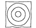Computer drawn lines are always totally straight, which can make them look unnatural and unfriendly. You can use Perlin Noise to introduce a wobblyness to a line drawing algorithm to make it appear as if it's been drawn by hand. You can also draw wobbly circles and boxes. Some research has been done on making a Sketchy User Interface. See: Creating Informal Looking Interfaces.

 

---

2 dimensional

Landscapes:	These are a perfect application for 2D Perlin Noise. Unlike the subdivision method, you do not have to store the landscape anywhere in memory, the height of any point on the landscape can be calculated easily. What's more, the land stretches indefinitely (almost), and can be calculated to minute detail, so it's perfect of variable level of detail rendering. The properties of the landscape can be defined easily too.
Clouds:	Again, cloud rendering is well suited to Perlin Noise.
Generating Textures:	All sorts of textures can be generated using Perlin Noise. See the table below for some examples. The textures generated can go on for ages before repeating (if ever), which makes them much more pleasant to look at than a repeating tiled texture map.

 

---

3 dimensional

3D Clouds:	You can, of course, produce volumetric clouds. You'll probably have to use some sort of ray tracing to visualise them.
Animated Clouds:	You can produce animated 2 dimensional clouds with 3D Perlin Noise, if you consider one dimension to be time.
Solid Textures:	Some rendering / raytracing programs, like POVray, apply texture to objects by literally carving them from a 3-dimensional texture. This was, the textures do not suffer from the warping usually associated with mapping 2D textures onto (non-flat) 3D objects.

 

---

4 dimensional

Animated 3D Textures and Clouds:

Moving into higher dimensions, you can easily produce animated clouds and solid textures. Just consider the extra dimension to be time.

 

---

Copyright Matt Fairclough 1998	The land, clouds and water in this picture were all mathematically generated with Perlin Noise, and rendered with Terragen.
	The clouds in this demo are animated with 3D perlin Noise. The algorithm had to be modified slightly to be able to produce Perlin Noise in real time. See the Clouds Article for more info on how this was done.

 

---

Generating Textures with Perlin Noise

Perlin is fantastic for generating textures. You can produce textures that are (for all practical purposes) infinitely large, but take up almost no memory. You can create marble, wood, swirly patterns, probably anything if you try hard. You can also define a 3D texture. You can think of this as a solid block of material, from which you can 'carve' an object. This allows you to produce textures which can be applied to any shaped object without distortion. It can take a lot of imagination, thought and experimentation to get a texture to look really good, but the results can be very impressive indeed.

 

Play around as much as you like. Use several Perlin functions to create a texture, try different persistences and different frequencies in different dimensions. You can use one Perlin function to affect the properties of another. Apply functions to their output. Do whatever you want, there's almost certainally a way to produce almost any texture you can dream up.

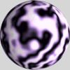
The following textures were made with 3D Perlin Noise

	Standard 3 dimensional perlin noise. 4 octaves, persistence 0.25 and 0.5
	Low persistence. You can create harder edges to the perlin noise by applying a function to the output.
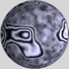	To create more interesting and complicated textures, you should try mixing several Perlin functions. This texture was created in two parts. Firstly a Perlin function with low persistence was used to define the shape of the blobs. The value of this function was used to select from two other functions, one of which defined the stripes, the other defined the blotchy pattern. A high value chose more of the former, a low value more of the latter. The stripes were defined by multiplying the first Perlin Function by some number (about 20) then taking the cosine.
	A marbly texture can be made by using a Perlin function as an offset to a cosine function.   texture = cosine( x + perlin(x,y,z) )
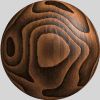
	Very nice wood textures can be defined. The grain is defined with a low persistence function like this: g = perlin(x,y,z) * 20 grain = g - int(g) The very fine bumps you can see on the wood are high frequency noise that has been stretched in one dimension. bumps = perlin(x*50, y*50, z*20) if bumps < .5 then bumps = 0 else bumps = 1t

 

---

References

Procedural textures: http://developer.intel.com/drg/mmx/appnotes/proctex.htm

Intel Developer Site article about using the new MMX technology to render Perlin Noise in real time.

Ken Perlin's Homepage: http://mrl.nyu.edu/perlin/

I assume the person responsable for Perlin Noise. He has an interesting page with lots of useful links to texturing and modeling stuff.

Texturing And Modeling A Procedural Approach: http://www.cs.umbc.edu/~ebert/book/book.html

Ken Perlin's book which goes in depth on using Perlin Noise, among other algorithms to generate textures and model various natural phenomena.

Procedural Texture Page: http://www.threedgraphics.com/pixelloom/tex_synth.html

This page is an attempt to collect any and all information and WWW links related to Procedural Texture Synthesis.