推荐系统 | 基础推荐模型 | GBDT+LR模型 | Python实现

---

基础推荐模型——传送门：

• 推荐系统 | 基础推荐模型 | 协同过滤 | UserCF与ItemCF的Python实现及优化
• 推荐系统 | 基础推荐模型 | 矩阵分解模型 | 隐语义模型 | PyTorch实现
• 推荐系统 | 基础推荐模型 | 逻辑回归模型 | LS-PLM | PyTorch实现
• 推荐系统 | 基础推荐模型 | 特征交叉 | FM | FFM | PyTorch实现
• 推荐系统 | 基础推荐模型 | GBDT+LR模型 | Python实现

---

一、GBDT+LR——特征工程模型化的开端

  FFM 模型采用引入特征域的方式增强了模型的特征交叉能力，但无论如何，FFM 只能做二阶的特征交叉，如果继续提高特征交叉的维度，会不可避免地产生组合爆炸和计算复杂度过高的问题。那么，有没有其他方法可以有效地处理高维特征组合和筛选的问题呢? 2014 年， Facebook 提出了基于 GBDT+ LR组合模型的解决方案。

1.GBDT+LR 组合模型的结构

  Facebook 提出了一种利用 GBDT 自动进行特征筛选和组合，进而生成新的离散特征向量，再把该特征向量当作 LR 模型输入，预估 CTR 的模型。其模型结构如下：

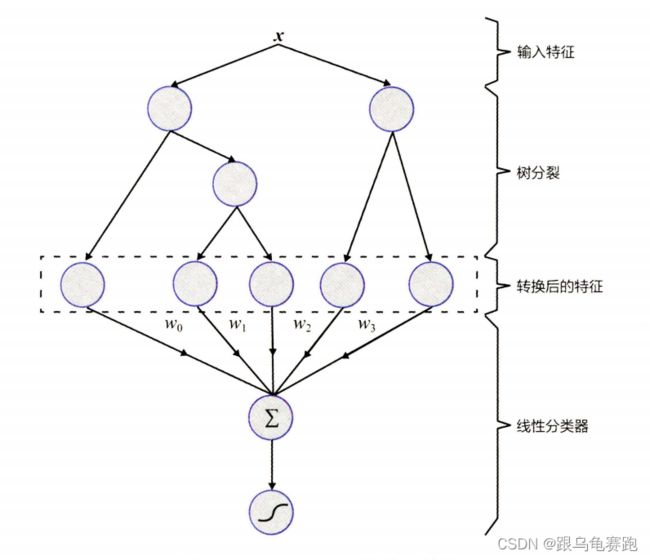
需要强调的是，用 GBDT 构建特征工程 ，利用 LR 预估 CTR 这两步是独立训练的，所以不存在如何将LR的梯度回传到GBDT 类复杂的问题。

2.GBDT 进行特征转换的过程

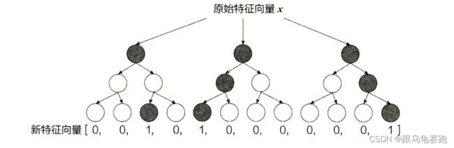
  利用训练集训练好 GBDT 模型之后，就可以利用该模型完成从原始特征向量到新的离散型特征向量的转化。具体过程为：一个训练样本在输入 GBDT 的某一子树后，会根据每个节点的规则最终落入某一叶子节点，把该叶子节点置为1 ，其他叶子节点置为0 ，所有叶子节点组成的向量即形成了该棵树的特征向量，把 GBDT 所有子树的特征向量连接起来，即形成了后续 LR 模型输入的离散型特征向量。
  举例来说，如下图所示，GBDT由三棵子树构成，每棵子树有4个叶子节点，输入一个训练样本后，其先后落入"子树1 "的第3个叶节点中，那么特征向量就是[0,0,1,0]，“子树 2” 的第1个叶节点，特征向量为 [1,0,0,0] ，"子树 3"的第4个叶节点，特征向量为 [0,0,01] ，最后连接所有特征向量，形成最终的特征向量[0,0,1,0,1,0,0,0,0,0,01]。

  事实上，决策树的深度决定了特征交叉的阶数。如果决策树的深度为 4，则通过3次节点分裂，最终的叶节点实际上是进行三阶特征组合后的结果，如此强的特征组合能力显然是 FM 系的模型不具备的。但 GBDT 容易产生过拟合，以及GBDT的特征转换方式实际上丢失了大量特征的数值信息，因此不能简单地说GBDT 的特征交叉能力强，效果就比FFM 好，在模型的选择和调试上，永远都是多种因素综合作用的结果。

3.GBDT+LR 组合模型开启特征工程新趋势

  GBDT+LR 组合模型对于推荐系统领域的重要性在于：它大大推进了特征工程模型化这一重要趋势。 GBDT+LR 组合模型出现之前，特征工程的主要解决方法有两个: 一是进行人工的或半人工的特征组合和特征筛选，二是通过改造目标函数，改进模型结构，增加特征交叉项的方式增强特征组合能力。但这两种方法都有弊端，第一种方法对算法工程师的经验和精力投入要求较高；第二种方法
则要求从根本上改变模型结构，对模型设计能力的要求较高。
  GBDT+LR 组合模型的提出，意味着特征工程可以完全交由一个独立的模型来完成，模型的输入可以是原始的特征向量 ，不必在特征工程上投入过多的人筛选和模型设计的精力，实现真正的端到端( End to End) 训练。
  广义上讲，深度学习模型通过各类网络结构 Embedding 层等方法完成特征工程的自动化，都是 GBDT+LR 开启的特征工程模型化这一趋势的延续。

二、GBDT+LR模型在criteo数据集上的实验

1.数据集介绍

  criteo数据集每行对应一个由 Criteo 提供的展示广告。有如下特征：

• Label：待预测广告，被点击是1，没有被点击是0
• I1-I13：共有 13 列数值型特征（主要是计数特征）
• C1-C26：共有 26 列类别型特征

数据集下载地址为：https://www.kaggle.com/c/criteo-display-ad-challenge/data。我这里采用前100k个样本进行实验。

2.Python实现

  FM推荐模型在criteo数据集上的Python实现，分为以下几个步骤：

• 数据预处理：dataProcess.py
• 数据加载：dataSet.py
• 模型搭建：LR_Model.py
• 主函数：训练及预测-main.py

2.1 数据预处理

#!usr/bin/env python
# -*- coding:utf-8 -*-
"""
@author: liujie
@file: dataProcess.py
@time: 2022/09/05
@desc:
    数据预处理流程：
        1.特征处理
        2.数据分割
"""
import torch
import numpy as np
import pandas as pd
from sklearn.preprocessing import LabelEncoder, OrdinalEncoder, KBinsDiscretizer
from sklearn.model_selection import train_test_split


class DataProcess():
    def __init__(self, file, nrows, sizes, device):
        # 特征列名
        names = ['label', 'I1', 'I2', 'I3', 'I4', 'I5', 'I6', 'I7', 'I8', 'I9', 'I10', 'I11',
                 'I12', 'I13', 'C1', 'C2', 'C3', 'C4', 'C5', 'C6', 'C7', 'C8', 'C9', 'C10', 'C11',
                 'C12', 'C13', 'C14', 'C15', 'C16', 'C17', 'C18', 'C19', 'C20', 'C21', 'C22',
                 'C23', 'C24', 'C25', 'C26']
        self.device = device
        # 读取数据
        self.data_df = pd.read_csv(file, sep="\t", names=names, nrows=nrows)
        self.data = self.feature_process()

    def feature_process(self):
        # 连续特征
        dense_features = ['I' + str(i) for i in range(1, 14)]
        # 离散特征
        sparse_features = ['C' + str(i) for i in range(1, 27)]
        features = dense_features + sparse_features

        # 缺失值填充:连续特征缺失值填充0；离散特征缺失值填充'-1'
        self.data_df[dense_features] = self.data_df[dense_features].fillna(0)
        self.data_df[sparse_features] = self.data_df[sparse_features].fillna('-1')

        # 连续特征等间隔分箱
        kb = KBinsDiscretizer(n_bins=100, encode='ordinal', strategy='uniform')
        self.data_df[dense_features] = kb.fit_transform(self.data_df[dense_features])

        # 特征进行连续编码，为了在与参数计算时使用索引的方式计算，而不是向量乘积
        ord = OrdinalEncoder()
        self.data_df[features] = ord.fit_transform(self.data_df[features])

        self.data = self.data_df[features + ['label']].values
        return self.data

    def train_valid_test_split(self, sizes):
        train_size, test_size = sizes[0], sizes[1]

        # 每一列的最大值加1
        field_dims = (self.data.max(axis=0).astype(int) + 1).tolist()[:-1]

        # 数据集分割为训练集、验证集、测试集
        train_data, test_data = train_test_split(self.data, train_size=train_size, random_state=2022)

        # 将ndarray格式转为tensor格式
        x_train = torch.tensor(train_data[:, :-1], dtype=torch.long)
        y_train = torch.tensor(train_data[:, -1], dtype=torch.float32)
        x_test = torch.tensor(test_data[:, :-1], dtype=torch.long)
        y_test = torch.tensor(test_data[:, -1], dtype=torch.float32)

        return field_dims, (x_train, y_train), (x_test, y_test)


if __name__ == '__main__':
    file = 'criteo-100k.txt'
    nrows = 100000
    sizes = [0.75, 0.25]
    device = torch.device("cuda" if torch.cuda.is_available() else "cpu")
    dataprocess = DataProcess(file, nrows, sizes, device)
    field_dims, (x_train, y_train), (x_test, y_test) \
        = dataprocess.train_valid_test_split(sizes)
    print(x_train.shape)
    print(field_dims)
    offsets = np.array((0, *np.cumsum(field_dims)[:-1]), dtype=np.long)
    print(offsets)

2.2 数据加载

#!usr/bin/env python
# -*- coding:utf-8 -*-
"""
@author: liujie
@file: dataSet.py
@time: 2022/09/05
@desc:构造加载数据集模块
"""
from torch.utils.data import Dataset


class My_DataSet(Dataset):
    def __init__(self, X, y):
        assert len(X) == len(y)
        self.X = X
        self.y = y

    def __len__(self):
        return len(self.X)

    def __getitem__(self, index):
        return self.X[index], self.y[index]

2.3 模型搭建

#!usr/bin/env python
# -*- coding:utf-8 -*-
"""
@author: liujie
@file: MLR_Model.py
@time: 2022/09/05
@desc:PyTorch实现LR模型
"""
import torch
import numpy as np
import torch.nn as nn


class LogisticRegression(nn.Module):
    def __init__(self, field_dims, emb_size):
        """
        :param field_dims: 特征数量列表，其和为总特征数量
        :param emb_size: embedding的维度
        """
        super(LogisticRegression, self).__init__()
        # embedding层
        self.emb = nn.Embedding(sum(field_dims), emb_size)
        # 模型初始化,针对激活函数：饱和函数，如Sigmoid，Tanh
        nn.init.xavier_uniform_(self.emb.weight.data)
        self.emb.weight.requires_grad = True
        # 偏置项
        self.offset = np.array((0, *np.cumsum(field_dims)[:-1]), dtype=np.long)
        # 可梯度更新
        self.bias = nn.Parameter(torch.zeros((1,)))

    def forward(self, x):
        """
        前向传播
        :param x: 输入数据,(batch,seq_len)
        :return:
        """
        x = x + x.new_tensor(self.offset)
        # (batch,seq_len) => (batch,seq_len,1) => (batch,1)
        x = self.emb(x).sum(1) + self.bias
        x = torch.sigmoid(x)
        return x

2.4 训练及预测

#!usr/bin/env python
# -*- coding:utf-8 -*-
"""
@author: liujie
@file: main.py
@time: 2022/09/05
@desc: GBDT+LR模型
"""

import tqdm
import torch
import numpy as np
import pandas as pd
import torch.nn as nn
from torch import optim
from LR_Model import LogisticRegression
from lightgbm import LGBMClassifier
from sklearn.preprocessing import OneHotEncoder
import matplotlib.pyplot as plt
from dataSet import My_DataSet
from torch.utils.data import DataLoader
from dataProcess import DataProcess
from sklearn.metrics import f1_score, recall_score, roc_auc_score

device = torch.device("cuda" if torch.cuda.is_available() else "cpu")
criteo_file = "criteo-100k.txt"
nrows = 100000
sizes = [0.75, 0.25]
embedding_size = 1
batch_size = 2048
num_epochs = 100
learning_rate = 1e-4
weight_decay = 1e-6


def train_and_test(train_dataloader, test_dataloader, model):
    # 损失函数
    criterion = nn.BCELoss()
    # 优化器
    optimizer = optim.Adam(model.parameters(), lr=learning_rate, weight_decay=weight_decay)
    # 记录训练与测试过程的损失，用于绘图
    train_loss, test_loss, train_acc, test_acc = [], [], [], []
    for epoch in range(num_epochs):
        train_loss_sum = 0.0
        train_len = 0
        train_correct = 0
        # 显示训练进度
        train_dataloader = tqdm.tqdm(train_dataloader)
        train_dataloader.set_description('[%s%04d/%04d]' % ('Epoch:', epoch + 1, num_epochs))

        # 训练模式
        model.train()
        model.to(device)
        for i, data_ in enumerate(train_dataloader):
            x, y = data_[0].to(device), data_[1].to(device)
            # 开始当前批次训练时，优化器的梯度置零，否则，梯度会累加
            optimizer.zero_grad()
            # output size = (batch,)
            output = model(x)
            loss = criterion(output.squeeze(1), y)
            # 反向传播
            loss.backward()
            # 利用优化器更新参数
            optimizer.step()
            # 默认reduction="mean",因此需要乘以个数
            train_loss_sum += loss.detach() * len(y)
            train_len += len(y)
            _, predicted = torch.max(output, 1)
            train_correct += (predicted == y).sum().item()
            # print("train_correct=\n", train_correct)
            # print("train_acc=\n", train_correct / train_len)
            F1 = f1_score(y.cpu(), predicted.cpu(), average="weighted")
            Recall = recall_score(y.cpu(), predicted.cpu(), average="micro")

            # 设置日志
            postfic = {"train_loss: {:.5f},train_acc:{:.3f}%,F1: {:.3f}%,Recall:{:.3f}%".
                           format(train_loss_sum / train_len, 100 * train_correct / train_len, 100 * F1, 100 * Recall)}
            train_dataloader.set_postfix(log=postfic)
        train_loss.append((train_loss_sum / train_len).item())
        train_acc.append(round(train_correct / train_len, 4))

        # 测试
        test_dataloader = tqdm.tqdm(test_dataloader)
        test_dataloader.set_description('[%s%04d/%04d]' % ('Epoch:', epoch + 1, num_epochs))
        model.eval()
        model.to(device)
        with torch.no_grad():
            test_loss_sum = 0.0
            test_len = 0
            test_correct = 0
            for i, data_ in enumerate(test_dataloader):
                x, y = data_[0].to(device), data_[1].to(device)
                output = model(x)
                loss = criterion(output.squeeze(1), y)
                test_loss_sum += loss.detach() * len(x)
                test_len += len(y)
                _, predicted = torch.max(output, 1)
                test_correct += (predicted == y).sum().item()
                F1 = f1_score(y.cpu(), predicted.cpu(), average="weighted")
                Recall = recall_score(y.cpu(), predicted.cpu(), average="micro")
                # 设置日志
                postfic = {"test_loss: {:.5f},test_acc:{:.3f}%,F1: {:.3f}%,Recall:{:.3f}%".
                               format(test_loss_sum / test_len, 100 * test_correct / test_len, 100 * F1, 100 * Recall)}
                test_dataloader.set_postfix(log=postfic)
            test_loss.append((test_loss_sum / test_len).item())
            test_acc.append(round(test_correct / test_len, 4))

    return train_loss, test_loss, train_acc, test_acc


def transform(lgbm, train_X, train_y, test_X, test_y):
    # One-hot Encoding
    ohe = OneHotEncoder()
    sparse_mat = ohe.fit_transform(np.vstack([train_X, test_X]))
    train_len, test_len = len(train_X), len(test_X)
    sparse_train_X = sparse_mat[:train_len]
    sparse_test_X = sparse_mat[-test_len:]

    # lgbm fit transoform
    lgbm.fit(sparse_train_X, train_y, eval_set=[(sparse_test_X, test_y)], verbose=100, early_stopping_rounds=100)
    # pred_leaf = True 表示返回每棵树的叶节点序号，并将新特征向量与原向量进行拼接
    fusion_train_X = np.hstack([lgbm.predict(sparse_train_X, pred_leaf=True), train_X])
    fusion_test_X = np.hstack([lgbm.predict(sparse_test_X, pred_leaf=True), test_X])
    # 叶节点序列对应的特征向量的最大值均为num_leaves
    fusion_field_dims = (np.vstack([fusion_train_X, fusion_test_X]).max(axis=0) + 1).tolist()

    fusion_train_X = torch.tensor(fusion_train_X, dtype=torch.long).to(device)
    fusion_test_X = torch.tensor(fusion_test_X, dtype=torch.long).to(device)
    return fusion_field_dims, fusion_train_X, fusion_test_X


def main():
    """
    主函数
    :return:
    """
    dataProcess = DataProcess(criteo_file, nrows, sizes, device)
    field_dims, (x_train, y_train), (x_test, y_test) \
        = dataProcess.train_valid_test_split(sizes)

    lgbm = LGBMClassifier(
        learning_rate=0.1,
        n_estimators=10230,
        num_leaves=31,
        max_depth=7,
        subsample=0.8,
        colsample_bytree=0.8,
        metric='auc',
        objective='binary'
    )

    # GBDT特征变换
    field_dims, x_train, x_test = transform(lgbm, x_train, y_train, x_test, y_test)
    # 构造数据集
    trainDataset = My_DataSet(x_train, y_train)
    train_dataloader = DataLoader(trainDataset, batch_size=batch_size, shuffle=True)

    testDataset = My_DataSet(x_test, y_test)
    test_dataloader = DataLoader(testDataset, batch_size=batch_size)
    # 模型实例化
    model = LogisticRegression(field_dims, embedding_size)

    # 训练与测试
    train_loss, test_loss, train_acc, test_acc = train_and_test(train_dataloader, test_dataloader, model)

    # 绘图，展示损失变化
    epochs = np.arange(num_epochs)
    plt.plot(epochs, train_loss, 'b-', label='Training loss')
    plt.plot(epochs, test_loss, 'r--', label='Validation loss')
    plt.title('Training And Validation Loss')
    plt.xlabel('Epochs')
    plt.ylabel('Loss')
    plt.legend()
    plt.show()

    epochs = np.arange(num_epochs)
    plt.plot(epochs, train_acc, 'b-', label='Training acc')
    plt.plot(epochs, test_acc, 'r--', label='Validation acc')
    plt.title('Training And Validation acc')
    plt.xlabel('Epochs')
    plt.ylabel('acc')
    plt.legend()
    plt.show()


if __name__ == '__main__':
    main()

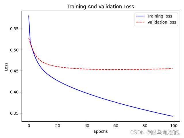
损失迭代图：

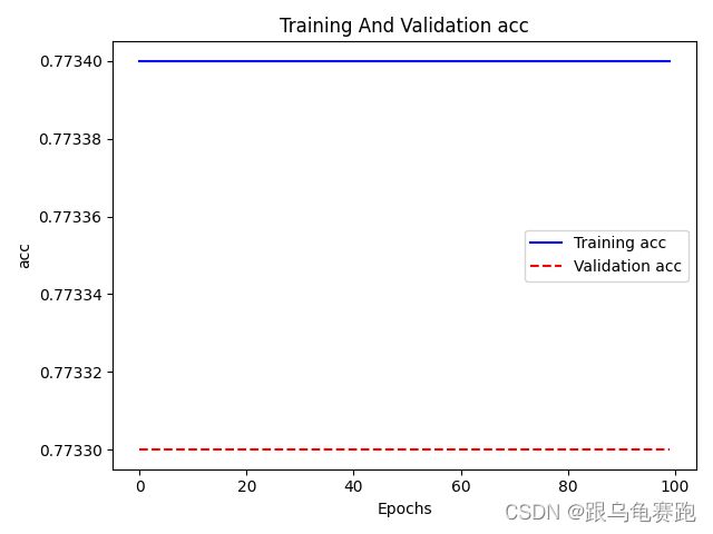
准确率迭代图：

---

参考：

• 《深度学习推荐系统》王喆
• Practical Lessons from Predicting Clicks on Ads at Facebook