BusterNet网络Python模型实现学习笔记一
实在是无力吐槽了,心力交瘁。作者Github仓库给了错误的 USCISI-CMFD-Small 数据集。自己捣鼓了半天,发现原来是压缩之后数据集,也就是 LMDB 文件格式出错了。实在是误人子弟,自己已经气急败坏了现在…
但是既然论文都花那么长时间看了,总归要学点东西,那就学一下他 net.py 文件是怎么写的吧。本篇文章还未完稿,和大家交流学习!
文章目录
-
- 一、`class Inception`
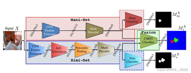
- 二、Mani-Det 层
- 三、Simi-Det 层
-
- 3.1 CNN Feature Extractor 层
- 3.2 Self-Correlation 层
- 3.3 Percentile Pooling 层
- 3.4 Mask Decoder 和 Binary Classifier 层
- 四、BusterNet 总体网络
- 五、主程序
一、class Inception
class Inception(nn.Module):
nn.Module是PyTorch中所有模型的基类。通过继承nn.Module,我们可以很方便地构建自己的模型。
    def __init__(self, in_channels, ch1x1, ch3x3red, ch3x3, ch5x5red, ch5x5, conv_block=None, is_last=False):
        super(Inception, self).__init__()
        if conv_block is None:
            conv_block = BasicConv2D
        if is_last:
            k_size1,  k_size2, k_size3 = 5, 7, 11
        else:
            k_size1,  k_size2, k_size3 = 1, 3, 5

        self.branch1 = conv_block(in_channels, ch1x1, kernel_size=k_size1)

        self.branch2 = nn.Sequential(
            conv_block(in_channels, ch3x3red, kernel_size=1),
            conv_block(ch3x3red, ch3x3, kernel_size=k_size2, padding=1)
        )

        self.branch3 = nn.Sequential(
            conv_block(in_channels, ch5x5red, kernel_size=1),
            conv_block(ch5x5red, ch5x5, kernel_size=k_size3, padding=1)#padding=1 表示在卷积操作时,在输入张量的边界上增加一层大小为 1 的填充层。
        )
可以看到和论文图片中的一致,一个 BN-Inception 中他生成了3个branch。

二、Mani-Det 层
class ManipulationNet(nn.Module):
    def __init__(self):
        super(ManipulationNet, self).__init__()
        # self.features = nn.Sequential(*make_layers(cfgs['C']))
        self.features = models.vgg16_bn().features[:-10]
        self.mask_decoder = MaskDecoder(512)
        self.classifier = nn.Sequential(
            Conv2d(6, 1, kernel_size=3),
            nn.Sigmoid()
        )

    def forward(self, x):
        x = self.features(x)
        x = self.mask_decoder(x)
        mask = self.classifier(x)
        return x, mask

Mask Decoder 层的代码如下所示
class DeconvBlock(nn.Module):
    def __init__(self, in_channels, out_channels):
        super(DeconvBlock, self).__init__()
        self.upsample = nn.UpsamplingBilinear2d(scale_factor=2)

        h_channels = out_channels // 2
        self.inception = Inception(in_channels, out_channels, h_channels, out_channels, h_channels, out_channels)

    def forward(self, x):
        x = self.upsample(x)
        x = self.inception(x)
        return x

class MaskDecoder(nn.Module):
    def __init__(self, in_channels=512):
        super(MaskDecoder, self).__init__()
        self.f16 = Inception(in_channels, 8, 4, 8, 4, 8)

        self.deconv_0 = DeconvBlock(24, 6)
        self.deconv_1 = DeconvBlock(18, 4)
        self.deconv_2 = DeconvBlock(12, 2)
        self.deconv_3 = DeconvBlock(6, 2)

        self.pred_mask = Inception(6, 2, 1, 2, 1, 2, is_last=True)

    def forward(self, x):
        f16 = self.f16(x)
        f32 = self.deconv_0(f16)
        f64 = self.deconv_1(f32)
        f128 = self.deconv_2(f64)
        f256 = self.deconv_3(f128)
        pred_mask = self.pred_mask(f256)

        return pred_mask
有几个很有趣的点我来解释一下,关于DeconvBlock。这是基本的解卷积盒。按照论文中的写法,我们会有 4 4 4个解卷积的盒,如下图。但这样的话怎么着都对不齐,所以论文复现这里应该是写反了DeconvBlock中unsample和inception层的顺序。
self.upsample层不会影响通道数量,所以我们将代码写成下面的形式
    def forward(self, x):
        x = self.inception(x)
        x = self.upsample(x)
        return x
这样一来就能和论文中的图对齐了。

我们将目光放到ManipulationNet中的一行
self.mask_decoder = MaskDecoder(512)
以及 MaskDecoder 定义中的一句
class MaskDecoder(nn.Module):
    def __init__(self, in_channels=512):
        super(MaskDecoder, self).__init__()
不免让人好奇,传入的参数512还有没有用?
当我们实例化 MaskDecoder 类并传入一个参数,例如 MaskDecoder(256),您指定的参数值将覆盖构造函数中的默认值。在这种情况下,in_channels 参数将变为256而不是默认的512。
三、Simi-Det 层
class SimilarityNet(nn.Module):
    def __init__(self):
        super(SimilarityNet, self).__init__()
        # self.features = nn.Sequential(*make_layers(cfgs['C']))
        self.features = models.vgg16_bn().features[:-10]
        self.correlation_per_pooling = CorrelationPercPooling(nb_pools=256)
        self.mask_decoder = MaskDecoder(256)
        self.classifier = nn.Sequential(
            Conv2d(6, 1, kernel_size=3),
            nn.Sigmoid()
        )

    def forward(self, x):
        x = self.features(x)
        x = self.correlation_per_pooling(x)
        x = self.mask_decoder(x)
        mask = self.classifier(x)
        return x, mask
3.1 CNN Feature Extractor 层
论文中提到我们是使用提前训练好的 VGG16 作为 CNN Feature Extractor。代码中我们是如何实现的呢?
self.features = models.vgg16_bn().features[:-10]
这行代码首先使用models.vgg16_bn()创建一个预训练的VGG-16网络,该网络包含批量归一化(BatchNorm)层。models.vgg16_bn()返回一个包含预训练权重的VGG-16模型对象。接下来,.features属性提取了该模型中的所有特征提取层,即卷积层、批量归一化层、激活函数和池化层。最后,通过使用[:-10]切片操作,我们去掉了最后10层,得到一个修改后的特征提取网络。
因此,self.features将存储一个去掉最后10层的预训练VGG-16特征提取网络,以便在新任务中进行微调或作为特征提取器使用。

f m X f_{m}^{X} fmX ( 16 × 16 × 512 ) (16\times16\times512) (16×16×512)是从 CNN Feature Extractor 网络中提取出来的 feature tensor。可以被视为 16 × 16 16\times 16 16×16 patch-like features。
个人是这么理解的,每个特征向量有512维,而每个特征代表了一个 16 × 16 16\times 16 16×16 大小的原图像区域。
3.2 Self-Correlation 层
Simi-Det 分支当中有个很重要的层是 Self-Correlation 层,我们来研究一下代码中是如何实现的。
ρ ( i , j ) = ( f ~ m X [ i ] ) T f ~ m X [ j ] / 512 (1) \rho(i, j)=\left(\tilde{f}_{m}^{X}[i]\right)^{T} \tilde{f}_{m}^{X}[j] / 512\tag1 ρ(i,j)=(f~mX[i])Tf~mX[j]/512(1)
这不显然就是矩阵中第 ( i , j ) (i,j) (i,j) 个元素么,所以我们可以用如下形式计算皮尔逊相关系数(Pearson correlation coefficient)。
[ ( f ~ m X [ 1 ] ) T ( f ~ m X [ 2 ] ) T ⋮ ( f ~ m X [ 256 ] ) T ] [ f ~ m X [ 1 ] , f ~ m X [ 2 ] , ⋯ , f ~ m X [ 256 ] ] \left[\begin{array}{c} \left(\tilde{f}_{m}^{X}[1]\right)^{T} \\ \left(\tilde{f}_{m}^{X}[2]\right)^{T} \\ \vdots \\ \left(\tilde{f}_{m}^{X}[256]\right)^{T} \end{array}\right] \left[\tilde{f}_{m}^{X}[1] , \tilde{f}_{m}^{X}[2], \cdots, \tilde{f}_{m}^{X}[256]\right] (f~mX[1])T(f~mX[2])T⋮(f~mX[256])T [f~mX[1],f~mX[2],⋯,f~mX[256]]
我们来看代码中是如何实现的:
        n_bsize, n_feats, n_cols, n_rows = x.shape #batchsize x512x16x16
        n_maps = n_cols * n_rows
        x_3d = x.reshape(n_bsize, n_feats, n_maps)#batchsize x512x256

        x_corr_3d = torch.matmul(x_3d.transpose(1, 2), x_3d) / n_feats#(n_bsize, n_maps, n_maps)
        x_corr = x_corr_3d.reshape(n_bsize, n_maps, n_cols, n_rows)#(n_bsize, n_maps, n_cols, n_rows)
结果 x_corr_3d 是一个形状为 (n_bsize, n_maps, n_maps) 的张量,表示每个批次中的特征映射区域之间的自相关。这个张量将在后续步骤中用于计算百分位池化。
这和论文中,Self-Correlation 生成一个分数向量 S X S^X SX of shape 16 × 16 × 256 16\times16\times256 16×16×256 是一致的。
其实个人认为这么说不太好,写成 S X S^X SX of shape 256 × 256 256\times256 256×256 会更容易接受一点。
S X [ i ] = [ ρ ( i , 0 ) , ⋯ , ρ ( i , j ) , ⋯ , ρ ( i , 255 ) ] (3) S^{X}[i]=[\rho(i, 0), \cdots, \rho(i, j), \cdots, \rho(i, 255)]\tag3 SX[i]=[ρ(i,0),⋯,ρ(i,j),⋯,ρ(i,255)](3)
因为这个公式里面 i i i 有256种取值的方式。
3.3 Percentile Pooling 层
我们先来看看论文中怎么说的,我们要先将 S X [ i ] S^{X}[i] SX[i] 降序排列,那么这个 monotonic decreasing curve 将会在某个值的时候会有突然的下降,如果图象是匹配的化(这说明我们的经过排序的分数向量,它包含有足够的信息来在未来阶段说明什么特征是匹配的)。
S ′ X [ i ] = sort ( S X [ i ] ) (4) S^{\prime X}[i]=\operatorname{sort}\left(S^{X}[i]\right)\tag4 S′X[i]=sort(SX[i])(4)
Percentile Pooling 首先会标准化排序后的分数向量 by only picking those scores at percentile ranks of interests。也就是说如果我们对百分比在 p k p_k pk 的 S X [ i ] S^{X}[i] SX[i] 数值感兴趣,我们计算 k ′ k^\prime k′
k ′ = round ( p k ⋅ ( L − 1 ) ) (6) k^{\prime}=\operatorname{round}\left(p_{k} \cdot(L-1)\right)\tag6 k′=round(pk⋅(L−1))(6)
这一系列的 S ′ X [ i ] [ k ′ ] S^{\prime X} [i]\left[k^{\prime }\right] S′X[i][k′] 最后变成 a pooled percentile score vector P X [ i ] P^X[i] PX[i]。
P X [ i ] [ k ] = S ′ X [ i ] [ k ′ ] (5) P^{X}[i][k]=S^{\prime X}[i]\left[k^{\prime }\right]\tag5 PX[i][k]=S′X[i][k′](5)
论文里说加入 Percentile Pooling 他认为会有两个优点
- 网络可以接受任意大小的图片,因为本来 S ′ X [ i ] S^{\prime X}[i] S′X[i] 中 i i i 的数量是取决于输入图片大小的,现在 Percentile Pooling 就只保留固定的 K K K 个 scores。
- 可以降低维度,因为只有一部分的 score vector 被保留了下来,减小计算量。
看一下代码中是如何实现的
        if self.nb_pools is not None:
            self.ranks = torch.floor(torch.linspace(0, n_maps -1, self.nb_pools)).type(torch.long)
        else:
            self.ranks = torch.range(1, n_maps, dtype=torch.long)

		x_f1st_pool = x_f1st_sort[self.ranks]
这行代码的作用是在区间 [0, n_maps - 1] 内生成等间隔的 self.nb_pools 个值,然后对这些值向下取整,最后将结果转换为长整数类型的张量(torch.long)。self.nb_pools 就是论文中的 K K K。论文中经过 Percentile Pooling 后固定分数向量维度为 100。

3.4 Mask Decoder 和 Binary Classifier 层
经过 Percentile Pooling 之后,我们使用 Mask Decoder 来逐渐 upsample 特征 P X ( 256 × 256 × 100 ) P^X(256\times 256\times 100) PX(256×256×100) 到原本的图像大小 d s X ( 256 × 256 × 6 ) d_s^X(256\times 256\times 6) dsX(256×256×6)。使用 Binary Classifier 来生成复制粘贴掩膜 M s X ( 256 × 256 × 1 ) M_s^X(256\times 256\times 1) MsX(256×256×1)。
class CorrelationPercPooling(nn.Module):
    '''Custom Self-Correlation Percentile Pooling Layer
    '''
    def __init__(self, nb_pools=256, **kwargs):
        super(CorrelationPercPooling, self).__init__()
        self.nb_pools = nb_pools

        n_maps = 16*16

        if self.nb_pools is not None:
            self.ranks = torch.floor(torch.linspace(0, n_maps -1, self.nb_pools)).type(torch.long)
        else:
            self.ranks = torch.range(1, n_maps, dtype=torch.long)

    def forward(self, x):
        '''
            x_shape: (n, c, h, w)
        '''
        n_bsize, n_feats, n_cols, n_rows = x.shape
        n_maps = n_cols * n_rows
        x_3d = x.reshape(n_bsize, n_feats, n_maps)

        x_corr_3d = torch.matmul(x_3d.transpose(1, 2), x_3d) / n_feats
        x_corr = x_corr_3d.reshape(n_bsize, n_maps, n_cols, n_rows)

        # ranks = ranks.to(devices)
        x_sort, _ = torch.topk(x_corr, k=n_maps, dim=1, sorted=True)

        x_f1st_sort = x_sort.permute(1, 2, 3, 0)
        x_f1st_pool = x_f1st_sort[self.ranks]
        x_pool = x_f1st_pool.permute(3, 0, 1, 2)

        return x_pool
四、BusterNet 总体网络
class BusterNet(nn.Module):
    def __init__(self, image_size):
        super(BusterNet, self).__init__()

        self.image_size = image_size

        self.manipulation_net = ManipulationNet()
        self.similarity_net = SimilarityNet()

        self.inception = nn.Sequential(
            Inception(12, 3, 3, 3, 3, 3),
            Conv2d(9, 3, kernel_size=3),
            nn.Softmax2d()
        )

    def forward(self, x):
        mani_feat, mani_output = self.manipulation_net(x)#mani_feat 是输出的的特征,mani_output是输出的二值掩膜
        simi_feat, simi_output = self.similarity_net(x)

        merged_feat = torch.cat([simi_feat, mani_feat], dim=1)#将两个分支的特征合并到一起

        x = self.inception(merged_feat)#将合并的特征通过一个inception层

        mask_out = F.interpolate(x, size=(self.image_size, self.image_size), mode='bilinear')
        return mask_out, mani_output, simi_output
五、主程序
if __name__ == "__main__":
    model = BusterNet(256)
    print(model)
    num_params = sum(p.numel() for p in model.parameters() if p.requires_grad)
    print(num_params)
BusterNet(256)是指输入图片大小是 256 × 256 256\times 256 256×256的。实际上,为了简化问题,我们所有的图像都是 256 × 256 × 3 256\times 256\times 3 256×256×3 的 RGB 图像。
综上所述,num_params存储了神经网络模型中可训练参数的总数。这对于评估模型的复杂性和计算资源需求非常有用。