因果推断14--DRNet论文和代码学习
目录
论文介绍
代码实现
DRNet
ReadMe
因果森林
论文介绍
因果推断3--DRNet(个人笔记)_万三豹的博客-CSDN博客
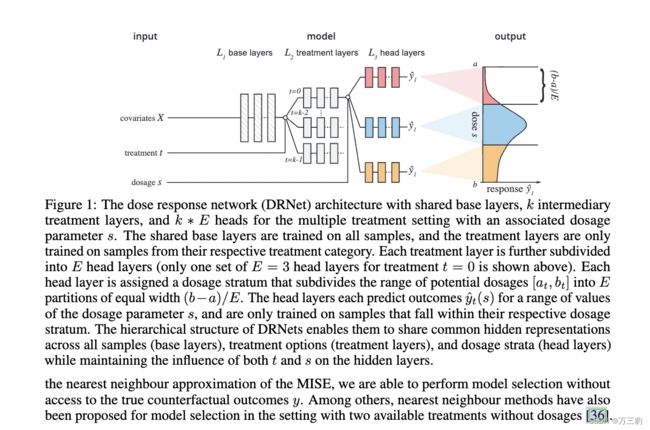
摘要:估计个体在不同程度的治疗暴露下的潜在反应,对于医疗保健、经济学和公共政策等几个重要领域具有很高的实际意义。然而,现有的从观察数据中估计反事实结果的学习方法要么专注于估计平均剂量-反应曲线,要么局限于只有两种没有相关剂量参数的治疗方法。在这里,我们提出了一种新的机器学习方法,用于学习反事实表示,用于使用神经网络估计具有连续剂量参数的任意数量治疗的单个剂量-反应曲线。在已建立的潜在结果框架的基础上,我们引入了性能指标、模型选择标准、模型架构和用于估计单个剂量反应曲线的开放基准。我们的实验表明,在这项工作中开发的方法在估计个体剂量反应方面设置了一个新的最先进的方法。
代码实现
GitHub - d909b/drnet: Dose response networks (DRNets) are a method for learning to estimate individual dose-response curves for multiple parametric treatments from observational data using neural networks.
DRNet
def get_method_name_map():
        return {
            'knn': KNearestNeighbours,
            'ols1': OrdinaryLeastSquares1,
            'ols2': OrdinaryLeastSquares2,
            'cf': CausalForest,
            'rf': RandomForest,
            'bart': BayesianAdditiveRegressionTrees,
            'nn': TFNeuralNetwork,
            'nn+': NeuralNetwork,
            'xgb': GradientBoostedTrees,
            'gp': GaussianProcess,
            'psm': PSM,
            'psmpbm': PSM_PBM,
            'ganite': GANITE,
            'gps': GPS,
        }
    def _build_graph(self, input_dim, num_units,
                     num_representation_layers, num_regression_layers, weight_initialisation_std,
                     reweight_sample=False, loss_function="l2",
                     imbalance_penalty_function="wass", rbf_sigma=0.1,
                     wass_lambda=10.0, wass_iterations=10, wass_bpt=True):
        """
        Constructs a TensorFlow subgraph for counterfactual regression.
        Sets the following member variables (to TF nodes):
        self.output         The output prediction "y"
        self.tot_loss       The total objective to minimize
        self.imb_loss       The imbalance term of the objective
        self.pred_loss      The prediction term of the objective
        self.weights_in     The input/representation layer weights
        self.weights_out    The output/post-representation layer weights
        self.weights_pred   The (linear) prediction layer weights
        self.h_rep          The layer of the penalized representation
        """
        ''' Initialize input placeholders '''
        self.x = tf.placeholder("float", shape=[None, input_dim], name='x')
        self.t = tf.placeholder("float", shape=[None, 1], name='t')
        self.y_ = tf.placeholder("float", shape=[None, 1], name='y_')

        ''' Parameter placeholders '''
        self.imbalance_loss_weight = tf.placeholder("float", name='r_alpha')
        self.l2_weight = tf.placeholder("float", name='r_lambda')
        self.dropout_representation = tf.placeholder("float", name='dropout_in')
        self.dropout_regression = tf.placeholder("float", name='dropout_out')
        self.p_t = tf.placeholder("float", name='p_treated')

        dim_input = input_dim
        dim_in = num_units
        dim_out = num_units

        weights_in, biases_in = [], []

        if num_representation_layers == 0:
            dim_in = dim_input
        if num_regression_layers == 0:
            dim_out = dim_in

        ''' Construct input/representation layers '''
        h_rep, weights_in, biases_in = build_mlp(self.x, num_representation_layers, dim_in,
                          self.dropout_representation, self.nonlinearity,
                          weight_initialisation_std=weight_initialisation_std)

        # Normalize representation.
        h_rep_norm = h_rep / safe_sqrt(tf.reduce_sum(tf.square(h_rep), axis=1, keep_dims=True))

        ''' Construct ouput layers '''
        y, y_concat, weights_out, weights_pred = self._build_output_graph(h_rep_norm, self.t, dim_in, dim_out,
                                                                          self.dropout_regression,
                                                                          num_regression_layers,
                                                                          weight_initialisation_std)

        ''' Compute sample reweighting '''
        if reweight_sample:
            w_t = self.t/(2*self.p_t)
            w_c = (1-self.t)/(2*(1-self.p_t))
            sample_weight = w_t + w_c
        else:
            sample_weight = 1.0

        self.sample_weight = sample_weight

        ''' Construct factual loss function '''
        if self.with_pehe_loss:
            risk = pred_error = tf.reduce_mean(sample_weight*tf.square(self.y_ - y)) + \
                                pehe_loss(self.y_, y_concat, self.t, self.x, self.num_treatments) / 10.
        elif loss_function == 'log':
            y = 0.995/(1.0+tf.exp(-y)) + 0.0025
            res = self.y_*tf.log(y) + (1.0-self.y_)*tf.log(1.0-y)

            risk = -tf.reduce_mean(sample_weight*res)
            pred_error = -tf.reduce_mean(res)
        else:
            risk = tf.reduce_mean(sample_weight*tf.square(self.y_ - y))
            pred_error = tf.sqrt(tf.reduce_mean(tf.square(self.y_ - y)))

        ''' Regularization '''
        for i in range(0, num_representation_layers):
            self.weight_decay_loss += tf.nn.l2_loss(weights_in[i])

        p_ipm = 0.5

        if self.imbalance_loss_weight_param == 0.0:
            imb_dist = tf.reduce_mean(self.t)
            imb_error = 0
        elif imbalance_penalty_function == 'mmd2_rbf':
            imb_dist = mmd2_rbf(h_rep_norm, self.t, p_ipm, rbf_sigma)
            imb_error = self.imbalance_loss_weight * imb_dist
        elif imbalance_penalty_function == 'mmd2_lin':
            imb_dist = mmd2_lin(h_rep_norm, self.t, p_ipm)
            imb_error = self.imbalance_loss_weight * mmd2_lin(h_rep_norm, self.t, p_ipm)
        elif imbalance_penalty_function == 'mmd_rbf':
            imb_dist = tf.abs(mmd2_rbf(h_rep_norm, self.t, p_ipm, rbf_sigma))
            imb_error = safe_sqrt(tf.square(self.imbalance_loss_weight) * imb_dist)
        elif imbalance_penalty_function == 'mmd_lin':
            imb_dist = mmd2_lin(h_rep_norm, self.t, p_ipm)
            imb_error = safe_sqrt(tf.square(self.imbalance_loss_weight) * imb_dist)
        elif imbalance_penalty_function == 'wass':
            imb_dist, imb_mat = wasserstein(h_rep_norm, self.t, p_ipm, sq=True,
                                            its=wass_iterations, lam=wass_lambda, backpropT=wass_bpt)
            imb_error = self.imbalance_loss_weight * imb_dist
            self.imb_mat = imb_mat  # FOR DEBUG
        elif imbalance_penalty_function == 'wass2':
            imb_dist, imb_mat = wasserstein(h_rep_norm, self.t, p_ipm, sq=True,
                                            its=wass_iterations, lam=wass_lambda, backpropT=wass_bpt)
            imb_error = self.imbalance_loss_weight * imb_dist
            self.imb_mat = imb_mat  # FOR DEBUG
        else:
            imb_dist = lindisc(h_rep_norm, p_ipm, self.t)
            imb_error = self.imbalance_loss_weight * imb_dist

        ''' Total error '''
        tot_error = risk
        if self.imbalance_loss_weight_param != 0.0:
            tot_error = tot_error + imb_error
        tot_error = tot_error + self.l2_weight*self.weight_decay_loss

        self.output = y
        self.tot_loss = tot_error
        self.imb_loss = imb_error
        self.imb_dist = imb_dist
        self.pred_loss = pred_error
        self.weights_in = weights_in
        self.weights_out = weights_out
        self.weights_pred = weights_pred
        self.h_rep = h_rep
        self.h_rep_norm = h_rep_norm
ReadMe
剂量反应网络(DRNets)是一种用于学习使用神经网络从观测数据估计多参数治疗的个体剂量反应曲线的方法。该存储库包含用于评估DRNets的源代码以及用于评估个体治疗效果的最相关的现有最先进方法(有关结果,请参阅我们的手稿)。为了便于将来的研究,源代码被设计为易于使用(1)新方法和(2)新的基准数据集进行扩展。
作者:Patrick Schwab,苏黎世[email protected]苏黎世联邦理工学院Lorenz [email protected],Stefan Bauer,MPI for Intelligent [email protected],苏黎世联邦理工学院Joachim [email protected]苏黎世联邦理工学院Walter [email protected]
许可证:MIT,请参阅License.txt
引用
如果您在工作中引用或使用我们的方法、代码或结果,请考虑引用:
@在过程中{schwab2020-剂量反应,
title={{学习用于估计个体剂量响应曲线的反事实表示}},
作者={施瓦布、帕特里克和林哈特、洛伦兹和鲍尔、斯特凡和布曼、约阿希姆·M和卡伦、沃尔特},
booktitle={{AAAI人工智能会议}},
年={2020}
}
用法:
可运行的脚本位于drnet/apps/子目录中。
drnet/apps/main.py是运行实验的主要可运行脚本。
drnet/apps/parameters.py中描述了可运行脚本的可用命令行参数
您可以通过将drnet/models/baseline/baseline.py子类化,将新的基线方法添加到评估中
有关如何实现自己的基线方法的示例,请参见drnet/models/baselines/neural_network.py。
通过向drnet/apps/main.py中的get_method_name_map方法添加新条目,可以从命令行注册新方法以供使用
您可以通过实现基准接口来添加新的基准,有关如何将自己的基准添加到基准套件的示例,请参见drnet/models/benchmarks。
通过向drnet/apps/evaluate.py中的get_benchmark_name_map方法添加新条目,可以从命令行注册新的基准测试以供使用
要求和相关性
该项目设计用于Python 2.7。我们不能保证,也没有测试过与Python 3的兼容性。
要运行TCGA和News基准,需要下载包含这些基准的原始数据样本的SQLite数据库(News.db和TCGA.db)。
您可以使用以下链接下载原始数据:tcga.db和news.db。
请注意,您需要大约10GB的可用磁盘空间来存储数据库。
将数据库文件保存到/数据目录,以便与下面的分步指南兼容或相应地调整命令。
要运行MVICU基准测试,您需要访问MIMIC-III数据库,由于数据集的敏感性,这需要经过审批过程。
注意,您需要大约75GB的可用磁盘空间来存储带有索引的MIMIC-III数据库。
访问数据集并将MIMIC-III数据加载到SQLite数据库(保存为例如/your/path/to/mimic3.db)后,可以使用drnet/apps/load_db_icu.py脚本将MVICU基准数据从MIMIC-IIII数据库提取到中的单独数据库中/数据文件夹,通过运行:
python drnet/apps/load_db_icu.py/your/path/to/mimic3.db./data
一旦建立,基准数据库将使用大约43MB的磁盘空间。
要运行BART、因果森林和GPS,并再现需要安装R的数字。看见https://www.r-project.org/安装说明。
要运行BART,需要安装R包rJava和bartMachine。看见https://github.com/kapelner/bartMachine安装说明。注意,rJava也需要一个工作的Java安装。
要运行因果森林,需要安装R包grf。看见https://github.com/grf-labs/grf安装说明。
要运行GPS,您需要安装R包causaldrf,例如在R-shell中运行install.packages(“causaldrv”)。
要复制论文的数字,您需要安装R-packagelatex2exp。看见https://cran.r-project.org/web/packages/latex2exp/vignettes/using-latex2exp.html安装说明。
有关python依赖关系,请参阅setup.py。您可以使用pipinstall。安装drnet包及其python依赖项。请注意,如果您的系统上没有正常的R安装,rpy2的安装将失败(请参见上文)。
再现实验
确保您具备上面列出的必要要求,包括/与此文件相关的数据目录以及所需的数据库(参见上文)。
您可以使用脚本drnet/apps/run_all_experiments.py获取main.py使用的精确参数,以重现论文中的实验结果。
drnet/apps/run_all_experiments.py脚本打印。
因果森林
https://grf-labs.github.io/grf/articles/grf.h
return self.grf.causal_forest(x,
                                      FloatVector([float(yy) for yy in y]),
                                      FloatVector([float(tt) for tt in t]), seed=909)
W
The treatment assignment (must be a binary or real numeric vector with no NAs).
W
治疗分配(必须是没有NA的二进制或实数矢量)。
class CausalForest(PickleableMixin, Baseline):
    def __init__(self):
        super(CausalForest, self).__init__()
        self.bart = None

    def install_grf(self):
        from rpy2.robjects.packages import importr
        import rpy2.robjects.packages as rpackages
        from rpy2.robjects.vectors import StrVector
        import rpy2.robjects as robjects

        # robjects.r.options(download_file_method='curl')

        # package_names = ["grf"]
        # utils = rpackages.importr('utils')
        # utils.chooseCRANmirror(ind=0)
        # utils.chooseCRANmirror(ind=0)
        #
        # names_to_install = [x for x in package_names if not rpackages.isinstalled(x)]
        # if len(names_to_install) > 0:
        #     utils.install_packages(StrVector(names_to_install))

        return importr("grf")

    def _build(self, **kwargs):
        from rpy2.robjects import numpy2ri
        from sklearn import linear_model
        grf = self.install_grf()

        self.grf = grf
        numpy2ri.activate()
        num_treatments = kwargs["num_treatments"]
        self.with_exposure = kwargs["with_exposure"]

        return [linear_model.Ridge(alpha=.5)] +\
               [None for _ in range(num_treatments)]

    def predict_for_model(self, model, x):
        base_y = Baseline.predict_for_model(self, self.model[0], x)
        if model == self.model[0]:
            return base_y
        else:
            import rpy2.robjects as robjects
            r = robjects.r
            result = r.predict(model, self.preprocess(x))
            y = np.array(result[0])
            return y[:, -1] + base_y

    def fit_grf_model(self, x, t, y):
        from rpy2.robjects.vectors import StrVector, FactorVector, FloatVector, IntVector
        return self.grf.causal_forest(x,
                                      FloatVector([float(yy) for yy in y]),
                                      FloatVector([float(tt) for tt in t]), seed=909)
参考:
- 《因果学习周刊》第8期:因果反事实预测 - 知乎
- 因果效应估计:用数据和模型指导决策 - 知乎