吴恩达机器学习作业笔记(线性回归)

零基础知识

1.DataFrame结构

Pandas DataFrame入门教程（图解版）
DataFrame 一个表格型的数据结构，既有行标签（index），又有列标签（columns），它也被称异构数据表，所谓异构，指的是表格中每列的数据类型可以不同，比如可以是字符串、整型或者浮点型等

pd.DataFrame( data, index, columns, dtype, copy)

data可以是多种类型
index和columns传入相应的一维数组作为标签，默认np.arange(n)，这里传入一维，不区分列表list和numpy的ndarray数组类型。
copy默认为false
1.1掌握一维列表与二维列表创建DataFrame结构

import pandas as pd
data = [1,2,3,4,5]
df = pd.DataFrame(data)
print(df)
输出如下
     0
0    1
1    2
2    3
3    4
4    5
import pandas as pd
data = [['Alex',10],['Bob',12],['Clarke',13]]
df = pd.DataFrame(data,columns=['Name','Age'],dtype=float)
print(df)
      Name     Age
0     Alex     10.0
1     Bob      12.0
2     Clarke   13.0

1.2了解字典创建DataFrame结构

import pandas as pd
data = {'Name':['Tom', 'Jack', 'Steve', 'Ricky'],'Age':[28,34,29,42]}
df = pd.DataFrame(data, index=['rank1','rank2','rank3','rank4'])
print(df)
输出如下
         Age    Name
rank1    28      Tom
rank2    34     Jack
rank3    29    Steve
rank4    42    Ricky

1.3Pandas csv读写文件

2.Numpy相关知识

NumPy ndarray对象

NumPy 定义了一个 n 维数组对象，简称 ndarray 对象，它是一个一系列相同类型元素组成的数组集合

2.1掌握创建ndarray对象，和.shape函数

import numpy

a=numpy.array([1,2,3])#使用列表构建一维数组
print(a)
[1 2 3]
print(type(a))
#ndarray数组类型
<class 'numpy.ndarray'>

b=numpy.array([[1,2,3],[4,5,6]])
print(b)
[[1 2 3]
[4 5 6]]

c=numpy.array([[1,2,3]])
print(a.shape)
输出(3,)
print(b.shape)
输出(2,3)
print(c.shape)
输出(1,3)

2.2掌握reshape数组变维

import numpy as np 
e = np.array([[1,2],[3,4],[5,6]]) 
print("原数组",e) 
e=e.reshape(2,3) 
print("新数组",e)  
原数组 
[[1 2]
[3 4]
[5 6]]
新数组
[[1 2 3]
[4 5 6]]

2.3数组的区间创建：

numpy.arange(start, stop, step, dtype)

不包含终止值

np.linspace(start, stop, num=50, endpoint=True, retstep=False, dtype=None)

形成num个均匀的样本，endpoint为False时不包含终止值

掌握numpy的索引与切片
通过冒号：来分割参数，[起始值：终止值：间隔]
np.hstack用法
np.hstack将参数元组的元素数组按水平方向进行叠加

2.4Numpy的矩阵乘法

X.dot(Y)
np.dot(X,Y)

numpy矩阵乘法中的multiply，matmul和dot

正文

import pandas as pd
import numpy as np
import matplotlib.pyplot as plt

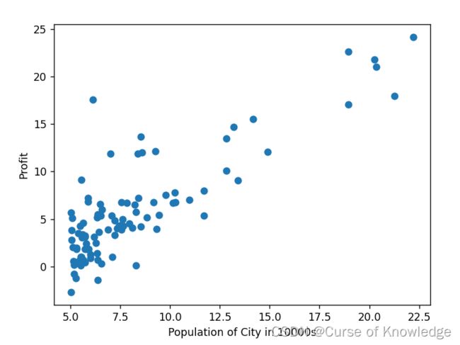
data = pd.read_csv("ex1data1.txt",names=["population","profit"])
print(data.head())
X = data.population
y = data.profit
plt.scatter(X,y)
plt.xlabel("Population of City in 10000s")
plt.ylabel("Profit")
plt.show()

data.head()输出前五行
population   profit
0      6.1101  17.5920
1      5.5277   9.1302
2      8.5186  13.6620
3      7.0032  11.8540
4      5.8598   6.8233

data = np.array(data)

把dataframe转化成了numpy数组

X = data[:,0].reshape(-1,1)
X = np.hstack([np.ones((len(X),1)),X])
y = data[:,1].reshape(-1,1)
theta = np.zeros(X.shape[1]).reshape(-1,1)

到这里，X，y，theta已经初始化完毕

X一个m行2列的矩阵，第一列代表x_0，全部是1，第二列是x_1，是数据Population

y是一个m行1列的矩阵，代表profit

theta代表两个参数

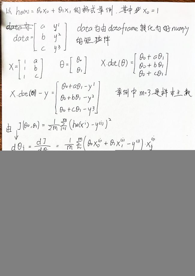
def J(X,y,theta):
    cost = np.sum((X.dot(theta)-y)**2)/(2*len(X))
    return cost

这是在定义Cost Function

def dJ(X,y,theta):
    ans =X.T.dot(X.dot(theta)-y) /len(X)
    return ans#返回一个(2,1)矩阵，表示dtheta0，dtheta1

这是在计算梯度，使用向量化语言，具体细节如下

def grad_descend(X,y,theta_init,learning_rate,iters,error):
    i=0
    theta = theta_init
    while i < iters:
        grad = dJ(X, y, theta)
        theta_old = theta
        theta = theta - learning_rate * grad
        if (abs(J(X,y,theta) - J(X,y,theta_old))) < error:
            print("第{}次梯度下降，达到理想误差".format(i+1))
            break
        i+=1
    return theta

定义梯度下降，当更新theta前后的Cost Function之差绝对值小于error的是时候停止循环
并返回此时的theta值，这就得到了两个参数

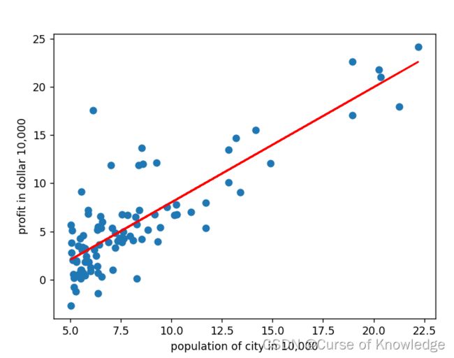
theta = grad_descend(X,y,theta,0.01,1e4,1e-8)
print(theta)

plt.scatter(data[:,0],data[:,1])
plt.plot(X[:,1],X.dot(theta),color="r")
plt.xlabel("population of city in 10,000")
plt.ylabel("profit in dollar 10,000")
plt.show()

输出
第3648次梯度下降,达到理想误差
[[-3.89027341]
 [ 1.19248036]]

总代码

import pandas as pd
import numpy as np
import matplotlib.pyplot as plt

data = pd.read_csv("D:\BaiduNetdiskDownload\data_sets\ex1data1.txt",names=["population","profit"])
print(data.head())
X = data.population
y = data.profit

data = np.array(data)#把dataframe转化成了numpy数组

X = data[:,0].reshape(-1,1)
X = np.hstack([np.ones((len(X),1)),X])
y = data[:,1].reshape(-1,1)



print("------------------------------------")
def J(X,y,theta):
    cost = np.sum((X.dot(theta)-y)**2)/(2*len(X))
    return cost
def dJ(X,y,theta):
    ans =X.T.dot(X.dot(theta)-y) /len(X)
    return ans#返回一个(2,1)矩阵，表示dtheta0，dtheta1
def grad_descend(X,y,theta_init,learning_rate,iters,error):
    i=0
    theta = theta_init
    while i < iters:
        grad = dJ(X, y, theta)
        theta_old = theta
        theta = theta - learning_rate * grad
        if (abs(J(X,y,theta) - J(X,y,theta_old))) < error:
            print("第{}次梯度下降,达到理想误差".format(i+1))
            break
        i+=1
    return theta
theta = np.zeros(X.shape[1]).reshape(-1,1)
theta = grad_descend(X,y,theta,0.01,1e4,1e-8)
print(theta)

plt.scatter(data[:,0],data[:,1])
plt.plot(X[:,1],X.dot(theta),color="r")
plt.xlabel("population of city in 10,000")
plt.ylabel("profit in dollar 10,000")
plt.show()

不使用正规方程

不适用正规方程的请情况下，可以分别计算每一个特征的梯度，最后组合到一个矩阵中。下面的dj0就代表theta0的梯度，dj1代表theta的梯度，观察dj0和dj1的表达式，他们的括号内的计算式是一样的，都是全部样本的X.dot(theta)-y的求和。

def dJ(X,y,theta):
    dj0 = 0
    dj1 = 0
    for i in range(len(X)):
        dj0 += (X[i].dot(theta) - y[i]) * X[i][0]
        dj1 += (X[i].dot(theta) - y[i]) * X[i][1]
    dj = np.hstack([dj0,dj1]).reshape(-1,1)
    return dj

检查梯度下降是否收敛

可以在grad_descend中的循环里加入以下语句，将每一次的Cost值保存到列表里，最后绘图，此时要将空列表传入函数体。

     temp=J(X, y, theta)
     listJ.append(temp)#将cost的值存到listJ中
     #使用append就省去初始化列表，一开始创建一个空列表，追加元素就可以
     #如果使用listJ[i] = temp，需要为列表提前开辟空间，但是这里的迭代次数还未知，不方便
     plt.plot(listJ)

多变量线性回归

这次使用numpy中的np.load()，直接导入数据，就是二维矩阵的形式。
在求解归一化时，是对特征X归一化，不对y进行处理。同时在验证数据时，验证集数据也要进行处理。
了解python中的广播，掌握

np.std(arr，axis = None)按列进行,计算指定数据 (数组元素)沿指定轴 (如果有)的标准偏差。
np.mean()
np.min() np.max()
np.subtract()矩阵相减

代码

import numpy as np
import matplotlib.pyplot as plt
data = np.loadtxt("ex1data2.txt",delimiter = ',')
X = data[:,0:2]
y = data[:,2].reshape(-1,1)

def norm(x):
    mean = np.mean(x,axis=0)
    #max = np.max(x,axis=0)
    #min = np.min(x, axis=0)
    #size = np.subtract(max,min)
    std = np.std(x,axis=0)
    norm = (x - mean)/std
    return mean,std,norm
mean,std,X = norm(X)

X = np.c_[np.ones(len(X)),X]

def J(X,y,theta):
    cost = np.sum((X.dot(theta)-y)**2)/(2*len(X))
    return cost
def dJ(X,y,theta):
    #xtheta = np.dot(X,theta)-y
    ans =X.T.dot(X.dot(theta)-y) /len(X)
    return ans#返回一个(2,1)矩阵，表示dtheta0，dtheta1
def grad_descend(X,y,theta_init,learning_rate,iters,error,listJ):
    i=0
    theta = theta_init
    while i < iters:
        grad = dJ(X, y, theta)
        temp=J(X, y, theta)
        listJ.append(temp)#将cost的值存到listJ中
        theta_old = theta
        theta = theta - learning_rate * grad
        if (abs(J(X,y,theta) - J(X,y,theta_old))) < error:
            print("第{}次梯度下降,达到理想误差".format(i+1))
            break
        i+=1
    return theta
listJ = []
theta = np.zeros(X.shape[1]).reshape(-1,1)
theta = grad_descend(X,y,theta,0.01,1e5,1e-8,listJ)
print(theta)
plt.plot(listJ)