时序分析 44 -- 时序数据转为空间数据 (三) 格拉姆角场 python 实践 （上）

格拉姆角场

python实践

    时序预测问题是一个古老的问题了，在笔者关于时序分析的系列中已经介绍了多种时序预测分析技术和方法。本篇我们将使用一种新的思路来进行时序预测：对金融数据进行GAF(格拉姆角场）编码成图像数据，后采用卷积神经网络对该金融时序数据进行预测。关于格拉姆角场的理论部分请参见笔者的另外一篇博文格拉姆角场
让我们开始吧。

导入所需库

import pandas as pd
import matplotlib
import matplotlib.pyplot as plt
import datetime as dt
import os
from pandas.tseries.holiday import USFederalHolidayCalendar as calendar
from multiprocessing import Pool
from mpl_toolkits.axes_grid1 import ImageGrid
from pyts.image import GramianAngularField
from typing import *
matplotlib.use('Agg')

读入数据

PATH = "G:\\financial_data\\IBM_adjusted.txt"
col_name = ['Date', 'Time', 'Open', 'High', 'Low','Close','Volume']
df = pd.read_csv(PATH, names=col_name, header=None)

df.head()

数据预处理

• 将数据聚合为一小时间隔
• 以0填充空值并移除重复值

def data_to_image_preprocess(df):
    """
    :return: None
    """
    # Drop unnecessary data
    df = df.drop(['High', 'Low', 'Volume'], axis=1)
    df['DateTime'] = pd.to_datetime(df['Date'] + ' ' + df['Time'], infer_datetime_format=True)
    df = df.groupby(pd.Grouper(key='DateTime', freq='1h')).mean().reset_index()
    df['Open'] = df['Open'].replace(to_replace=0, method='ffill')
    return df
    # Remove non trading days and times
    #clean_df = clean_non_trading_times(df)
    # Send to slicing
    #set_gaf_data(clean_df)

df = data_to_image_preprocess(df)
df.head()

清洗数据

• 移除周末、节假日和非交易时间（市场在上午9：30开放）

def clean_non_trading_times(df):
    """
    :param df: Data with weekends and holidays
    :return trading_data:
    """
    # Weekends go out
    df = df[df['DateTime'].dt.weekday < 5].reset_index(drop=True)
    df = df.set_index('DateTime')
    # Remove non trading hours
    df = df.between_time('9:00','16:00')
    df.reset_index(inplace=True)
    # Holiday days we want to delete from data
    holidays = calendar().holidays(start='2000-01-01', end='2020-12-31')
    m = df['DateTime'].isin(holidays)
    clean_df = df[~m].copy()
    trading_data = clean_df.fillna(method='ffill')
    return trading_data

clean_df = clean_non_trading_times(df)
clean_df.head()

def set_gaf_data(df):
    """
    :param df: DataFrame data
    :return: None
    """
    dates = df['DateTime'].dt.date
    dates = dates.drop_duplicates()
    list_dates = dates.apply(str).tolist()
    index = 20 #rows of data used on each GAF
    # Container to store data for the creation of GAF
    decision_map = {key: [] for key in ['LONG', 'SHORT']}
    while True:
        if index >= len(list_dates) - 1:
            break
        # Select appropriate timeframe
        data_slice = df.loc[(df['DateTime'] > list_dates[index - 20]) & (df['DateTime'] < list_dates[index])]
        gafs = []
        # Group data_slice by time frequency
        for freq in ['1h', '2h', '4h', '1d']:
            group_dt = data_slice.groupby(pd.Grouper(key='DateTime', freq=freq)).mean().reset_index()
            group_dt = group_dt.dropna()
            gafs.append(group_dt['Close'].tail(20))
        # Decide what trading position we should take on that day
        future_value = df[df['DateTime'].dt.date.astype(str) == list_dates[index]]['Close'].iloc[-1]
        current_value = data_slice['Close'].iloc[-1]
        decision = trading_action(future_close=future_value, current_close=current_value)
        decision_map[decision].append([list_dates[index - 1], gafs])
        index += 1
    print('GENERATING IMAGES')
    # Generate the images from processed data_slice
    generate_gaf(decision_map)
    # Log stuff
    dt_points = dates.shape[0]
    total_short = len(decision_map['SHORT'])
    total_long = len(decision_map['LONG'])
    images_created = total_short + total_long
    print("========PREPROCESS REPORT========:\nTotal Data Points: {0}\nTotal Images Created: {1}"
          "\nTotal LONG positions: {2}\nTotal SHORT positions: {3}".format(dt_points,
                                                                           images_created,
                                                                           total_short,
                                                                           total_long))

根据格拉姆角场我们所介绍的格拉姆角场的原理，我们需要将此时序数据转换为GAF矩阵，并进行两类预测：长期和短期。

set_gaf_data函数用来生成GAF图像。将时间序列聚合为四个不同时间间隔，且分别收集其最后的20行。每个聚合结果会产生一个图像。

def trading_action(future_close: int, current_close: int) -> str:
    """
    :param future_close: Integer
    :param current_close: Integer
    :return: Folder destination as String
    """
    current_close = current_close
    future_close = future_close
    if current_close < future_close:
        decision = 'LONG'
    else:
        decision = 'SHORT'
    return decision

交易日的最后一个数据点做出交易决策，如果下一天的收盘价高于当天则做多；反之则做空。

def create_gaf(ts):
    """
    :param ts:
    :return:
    """
    data = dict()
    gadf = GramianAngularField(method='difference', image_size=ts.shape[0])
    data['gadf'] = gadf.fit_transform(pd.DataFrame(ts).T)[0] # ts.T)
    return data

处理过的数据将会被传入上面的封装函数来生成GAF,此函数封装了pyts包中的GramianAngularField类的实例，它将首先将数据尺度缩放到[-1,1]之间，创建每一个$(X_i,X_j)$的时间相关性，然后计算极坐标。
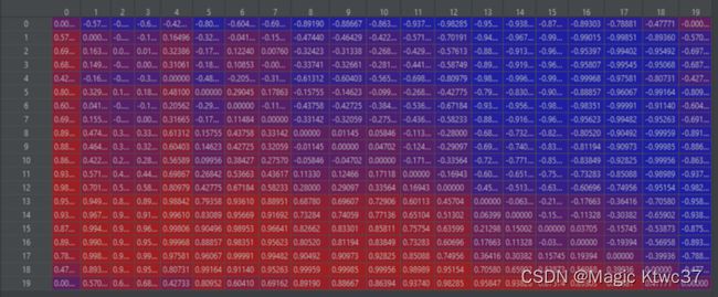
每一个聚合的时间序列会被转换为一个$N\times N$的矩阵，这里$N=20$。

转换后的矩阵采样如下图：

def generate_gaf(images_data: Dict[str, pd.DataFrame]) -> None:
    """
    :param images_data:
    :return:
    """
    for decision, data in images_data.items():
        for image_data in data:
            to_plot = [create_gaf(x)['gadf'] for x in image_data[1]]
            create_images(X_plots=to_plot,
                          image_name='{0}'.format(image_data[0].replace('-', '_')),
                          destination=decision)

def create_images(X_plots: Any, image_name: str, destination: str, image_matrix: tuple =(2, 2)) -> None:
    """
    :param X_plots:
    :param image_name:
    :param destination:
    :param image_matrix:
    :return:
    """
    fig = plt.figure(figsize=[img * 4 for img in image_matrix])
    grid = ImageGrid(fig,
                     111,
                     axes_pad=0,
                     nrows_ncols=image_matrix,
                     share_all=True,
                     )
    images = X_plots
    for image, ax in zip(images, grid):
        ax.set_xticks([])
        ax.set_yticks([])
        ax.imshow(image, cmap='rainbow', origin='lower')

    repo = os.path.join('G:\\financial_data\\TRAIN', destination)
    fig.savefig(os.path.join(repo, image_name))
    plt.close(fig)

print(dt.datetime.now())
print('CONVERTING TIME-SERIES TO IMAGES')
set_gaf_data(clean_df)
print('DONE!')
print(dt.datetime.now())

2022-09-13 23:51:05.377794
CONVERTING TIME-SERIES TO IMAGES
GENERATING IMAGES
PREPROCESS REPORT:
Total Data Points: 6340
Total Images Created: 6319
Total LONG positions: 3210
Total SHORT positions: 3109
DONE!
2022-09-14 00:23:05.449160

随机选取四个图像展示如下：

未完待续…