Winograd算法实现卷积原理

ref

Fast Algorithms for Convolutional Neural Networks

Fast Convolution based on Winograd Minimum Filtering: Introduction and Development

Efficient Winograd or Cook-Toom Convolution Kernel Implementation on Widely Used Mobile CPUs: https://arxiv.org/abs/1903.01521

https://www.emc2-ai.org/assets/docs/hpca-19/paper1-presentation.pdf

Performance Evaluation of INT8 Quantized Inference on Mobile GPUs

本文整理和改编自上述文献。

一维Winograd卷积

一维的输入向量d = [d0, d1, d2, d3] 与一维的向量filter g = [g0, g1, g3]进行卷积(更长的输入通过分段实现)，原始的计算方法为直接卷积，进行两次长度为3的向量内积，而Winograd的F(2, 3)快速计算方法（2指输出的元素个数，3指filter大小）为: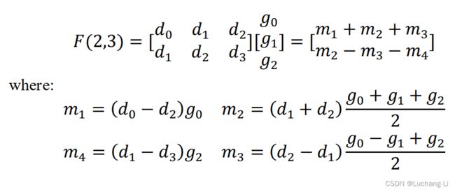

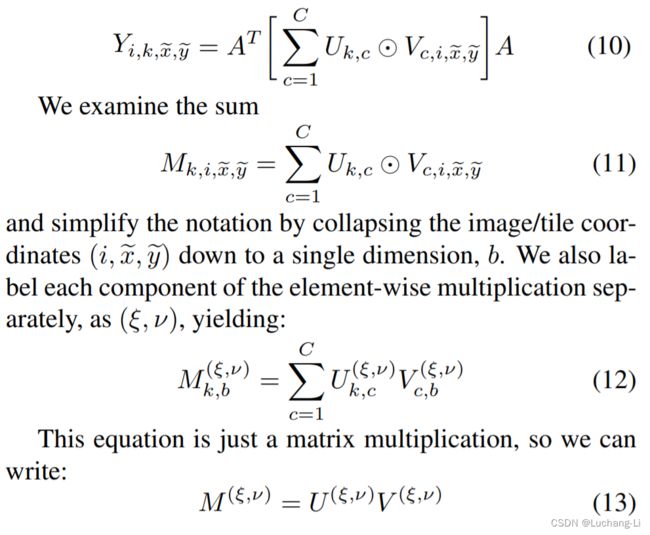
之所以能快速计算，原因是两次计算输入有重叠元素并且filter不变。

This algorithm uses just 4 multiplications and is therefore minimal by the formula µ(F(2, 3)) = 2 + 3 − 1 = 4. It also uses 4 additions involving the data, 3 additions and 2 multiplications by a constant involving the filter (the sum g0 + g2 can be computed just once), and 4 additions to reduce the products to the final result. 

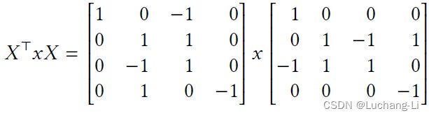
这个过程可以通过矩阵计算来进行描述：

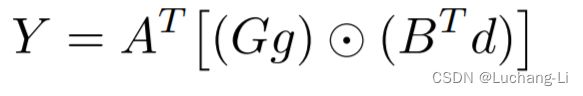
并且

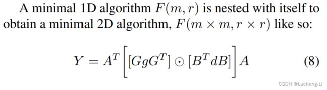
扩展到2D情形

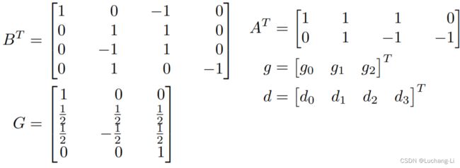
g is an r × r filter, d is an (m + r - 1) × (m + r - 1) input image tile.  is the filter transformation matrix, is the data transformation matrix. ⊙ is the corresponding bit multiplication of the matrix (Hadamard product), represents the output transformation matrix.

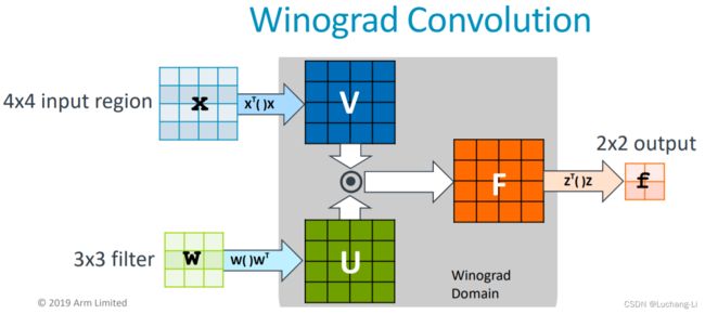
We can naturally split Winograd convolution into four separate stages:

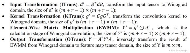
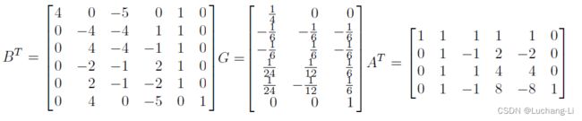
对于m=2, r=3, F(2x2,3x3)，g为3x3 filter，d为4x4 image tile，winograd domain点乘的矩阵大小为4x4，输出大小为2x2。F(2x2,3x3)在Arm的文档中表述为F(2x2, 3x3, 4x4)，括号里面三个量分布表示的是output, filter, input的shape，如F(2x2, 3x3, 4x4), F(3x3, 3x3, 5x5), F(2x2, 5x5, 6x6)。

Algorithms for F(m×m, r×r) can be used to compute convnet layers with r × r kernels. Each image channel is divided into tiles of size (m+r−1)×(m+r−1), with r−1 elements of overlap between neighboring tiles, yielding P = ⌈H/m⌉⌈W/m⌉ tiles per channel, C. F(m×m, r×r) is then computed for each tile and filter combination in each channel, and the results are summed over all channels. 

计算性能提升评估

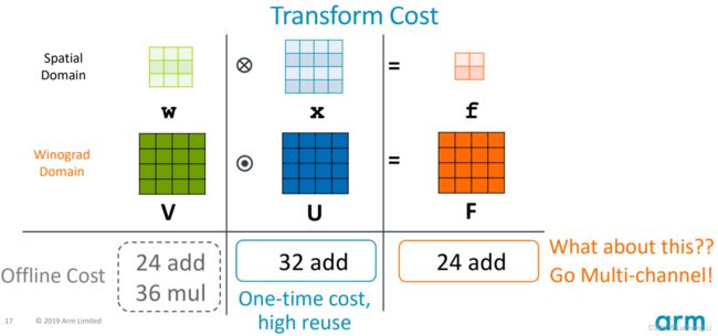
F(2×2, 3×3) uses 4×4 = 16 multiplications (两个4x4矩阵的elemwise乘法), whereas the standard algorithm uses 2 × 2 × 3 × 3 = 36. This is an arithmetic complexity reduction of 36/16 = 2.25.

The data transform uses 32 additions (由于B矩阵内容的特殊性，data transform只需要加法计算，filter 和inverse transform同理),

the filter transform uses 28 floating point instructions (推理场景filter固定的情况下这一步还可以提前算好), and the inverse transform uses 24 additions.

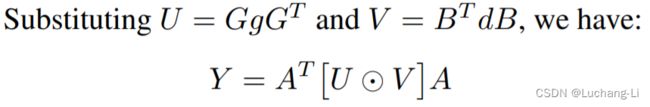
（arm的这个ppt里面，U, V含义与上面公式是反的）

K filters, C channels, batch N的处理

上面算法的基本思路是对一个通道的输入图像与一个通道filter进行计算得到，实际上每张图像需要与K个C个通道的filter进行上述计算，并且每次有batch=N张输入图像需要进行计算。

Thus we can reduce over C channels in transform space, and only then apply the inverse transform A to the sum. This amortizes the cost of the inverse transform over the number of channels. 也就是说每个C通道的卷积的inverse/output transform可以等到所有通道计算完成后计算一次，而不是每个通道的单张图像计算一次，如下图所示。

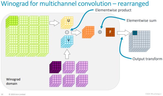
注意不是U与V直接做矩阵乘，而是在channel方向做矩阵乘！！！

多个batch和输出channel计算合并成矩阵计算： 

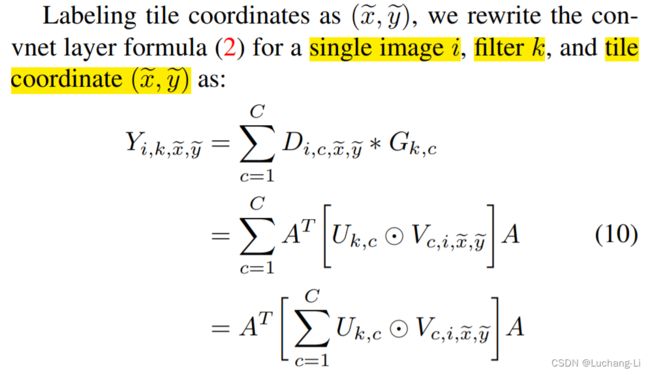
注意写在等号前面的符号上下标是需要在其范围内进行循环得到每个位置的结果，例如(ξ, ν)是在点乘的矩阵范围内循环从而得到点乘矩阵每个元素位置的结果。而k, b则是分别在K个output channel和batch=N范围内循环，从而得到整个output channel和batch的结果。而公式12到13的M和U, V省略了k, b等下标，是指M和U, V代表了整个K和batch，而不是单个索引位置的结果。

由于每个channel的图像是4x4图像点乘，整个C通道会4X4图像每个元素位置沿着通道方向累加求和，因此实际上每个元素位置是一个长度为C的向量内积（一维向量矩阵乘）。同时由于有K个输出通道，因此变成了N个C通道的input data与K个C通道的filter向量做矩阵乘。

这里公式的M和U, V是三个二维tensor，指的是做点乘的矩阵在每个元素坐标处的矩阵乘（因为实际上整个计算结果有N*K个点乘矩阵，也就是点乘的矩阵每个像素对应N*K个结果），如下图所示(同一种计算的两种表示方式而已)。而整个4x4点乘矩阵的所有位置的计算一起为一个16 batched matrix multiplies.

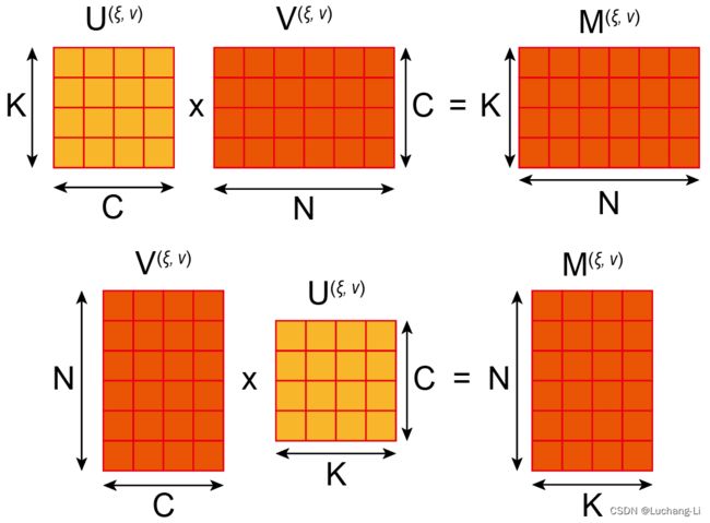
V矩阵在(ξ, ν)的内容为不同batch input data在data transform后点乘矩阵(ξ, ν)坐标处的内容。

U矩阵在(ξ, ν)的内容为K个filter在filter transform后点乘矩阵(ξ, ν)坐标处的内容。

具体实现算法

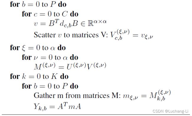
Fast Algorithms for Convolutional Neural Networks的实现算法

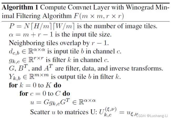
前两个for循环组读取data和filter的tile，然后进行transform（这里的transform虽然是矩阵乘的表达，但并不需要实际采用矩阵乘计算），Scatter u和v to matrices也就是U和V对于每个元素坐标把[batch, in channel]和[in channel, output channel]的矩阵数据放在最内层维度。

第三个for循环组对点乘矩阵每个元素位置的数据做矩阵乘，第四个for循环组把M从HW维度解释并且做output transform。

Fast Algorithms for Convolutional Neural Networks的GPU实现描述

The data and filter transform, 16 batched matrix multiplies (GEMMs), and inverse transform are all computed in the same block. The 16 batched GEMMs compute 32×32 outputs, which enables us to fit the workspace in the registers and shared memory of a single block and still have 2 active blocks per SM for latency hiding. Zero padding is implicit through use of predicates. If the predicate deselects a global image load, the zero value is loaded with a dual issued I2I instruction. Another resource limit is the instruction cache, which can only fit about 720 instructions. Our main loop is larger than this, but aligning the start of the loop with the 128 byte instruction cache-line boundary helps mitigate the cost of a cache miss.

We also implemented a variant that we call “FX” that runs a filter transform kernel first and stores the result in a workspace buffer. In general, we found that the FX variant of our implementation performed best unless the number of filters and channels was very large.

Image data is stored in CHWN order to facilitate contiguous and aligned memory loads, significantly reducing over-fetch. We employ a “super blocking” strategy to load 32 tiles of size 4×4 from a configurable number of images, rows, and columns. For N >= 32, we load tiles from 32 separate images. For N < 32, we load a super block of X × Y = 32/N tiles per image. This strategy facilitates efficient loads with small batch sizes, as theW×N dimensions of the input data are contiguous in memory. Furthermore, the 2 pixel overlap between adjacent tiles causes high L1 cache hit rates when using several tiles in a super block.

We also employ L2 cache blocking to increase the re-use of overlapping blocks. Since the number of image tiles is typically much larger than the number of filters, our block mapping iterates over a group of up to 128 filters in the inner loop, and then iterates over all image tiles in the second loop. All channels of the filter group fit in L2 cache, so each filter will only be loaded once from DDR memory, and each image tile will be loaded ⌈K/128⌉ times as we iterate over the filter groups. This strategy reduces DDR memory bandwidth by almost half.

这个CHWN格式比较奇特，一般很少用这种格式，常用是NCHW或者NHWC或者NC1HWC0。

ARM的实现

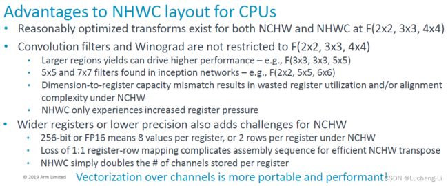
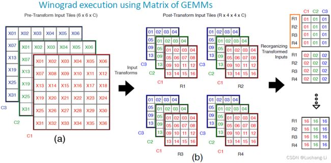
这个图是输入数据的读取和重排布，Arm采用了NHWC格式，在应对不同数据类型，tile大小等场景时相比NCHW格式具有明显的优势。

R指的是不同tile或者batch，C指的是input channel。对于batch=1时读取了6x6的子区域，由于2 pixels overlap, 拆分成了4个tile，相当于batch=4的计算。最终把数据重排布了HWNCi的格式便于后续做矩阵乘。（同样读取4个tile，读取1x4个而不是2x2个tile可能更有利于cache？）。

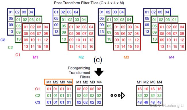
M指的是output channel，C指的是input channel。这里把weight数据重排布为HWCiCo格式。

接下来进行16个矩阵乘 ：

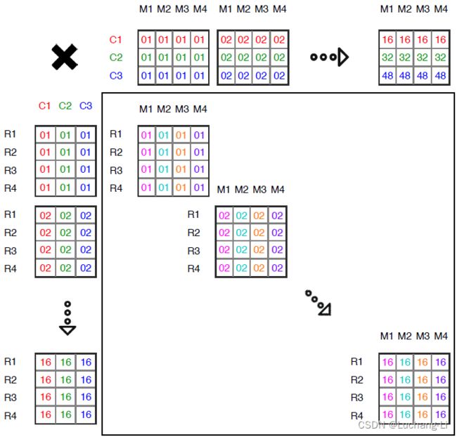
矩阵乘是HWNCi与HWCiCo进行batch矩阵乘，结果大小为HWNCo。仔细对照上面U, V矩阵乘的示例图，跟这里其实是一模一样的。因为是同一个点乘矩阵位置处每个batch的Ci通道输入数据与K个Ci通道的filter做矩阵乘。 

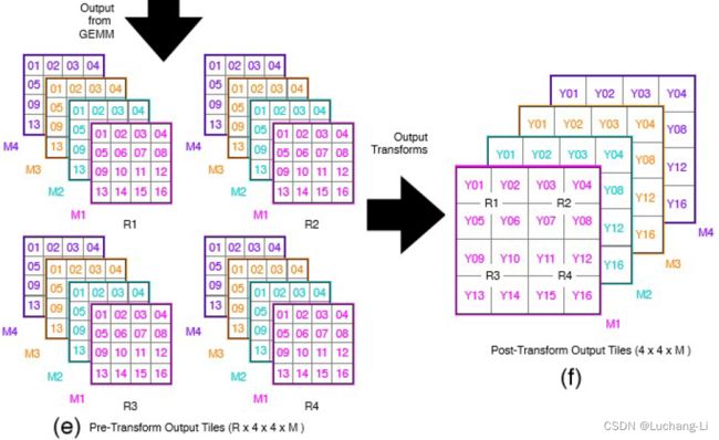
最后数据再重排布做output transform：

另一个全过程可视化图[Sparse Winograd Convolutional neural networks on small-scale systolic arrays]：

做矩阵乘的时候两个矩阵都是把C放在最内层，也就是NC格式。transform是对每个HW矩阵部分坐标之间的元素进行计算，例如input transform：

对读取后的数据x部分坐标数据进行加减操作，由于每个通道都要进行这样的独立操作，以NHWC格式读取后不同channel的数据对C通道可以采用向量计算完成。

扩展到其他tile大小的性能和数值精度

更大的tile和filter大小如F(4x4,3x3)

Applying the nesting formula yields a minimal algorithm for F(4 × 4, 3 × 3) that uses 6 × 6 = 36 multiplies, while the standard algorithm uses 4 × 4 × 3 × 3 = 144. This is an arithmetic complexity reduction of 4.

The 2D data transform uses 12(6 + 6) = 144 floating point instructions, the filter transform uses 8(3 + 6) = 72, and the inverse transform uses 10(6 + 4) = 100.

The number of additions and constant multiplications required by the minimal Winograd transforms increases quadratically with the tile size [10, p. 211]. Thus for large tiles, the complexity of the transforms will overwhelm any savings in the number of multiplications.

The magnitude of the transform matrix elements also increases with increasing tile size. This effectively reduces the numeric accuracy of the computation, so that for large tiles, the transforms cannot be computed accurately [16, p. 28].

As the number of multiplications is larger in F(4×4, 3×3) than in F(2 × 2, 3 × 3), Winograd convolution achieves 4× reduction in multiplication operations for F(4 × 4, 3 × 3), whereas 2.25× reduction for F(2×2, 3×3). In contrast, since the denominator in the G matrix is larger in F(4 × 4, 3 × 3) than F(2 × 2, 3 × 3), convolution computation errors using the former tend to be larger than the latter [42]. On the other hand, Winograd convolution requires more memory space to store transformed results [43].

Winograd convolution has only been applied to the 3 × 3 convolution kernel and small input tiles for a long time, because of the inherent numerical instability in the Winograd convolution calculation. When applied to larger convolution kernels or input tiles, the polynomial coefficients of the Winograd transform increase exponentially. This imbalance will be reflected in the elements of the transformation matrix, resulting in large relative errors. [7] studied that the source of this numerical instability is the large-scale Vandermonde matrix in the transformation [3] and proposed carefully selecting the corresponding polynomials that exhibit the smallest exponential growth. They also proposed scaling the transformation matrix to alleviate numerical instability. [23] used higher-order polynomials to reduce the error of Winograd convolution, but the cost was an increase in the number of multiplications. [42] handed over the processing of numerical errors to training to learn better convolution kernel weights and quantization in Winograd convolution. [51] proved mathematically that large convolution kernels can be solved by overlap and addition. [20], [52] solved large-size convolution kernel and non-unit step convolution into small convolution kernels to solve the numerical accuracy problem. [53] selected the appropriate output tile size based on symbolic calculation and meta-programming automation to balance numerical stability and efficiency. [54] proved that the floating-point calculation order in linear transformation affects accuracy, rearranged the calculation order in linear transformation based on Huffman coding, and proposed a mixed-precision algorithm.

这个tile大小并不是越大越好，tile大理论提升的性能更大，但是内部计算的矩阵乘shape更大，对资源要求更高，transform需要的额外计算也更多，可能抵消乘法数量降低的优势。此外，transform matrix的元素值更大，可能导致计算精度明显下降。具体性能精度可能要实际测试来选择使用。