【机器学习】集成学习（实战）

集成学习（实战）

实战部分将结合着 理论部分 进行，旨在帮助理解和强化实操（以下代码将基于 jupyter notebook 进行）。

---

一、准备工作（设置 jupyter notebook 中的字体大小样式等）

import numpy as np
import os
%matplotlib inline
import matplotlib
import matplotlib. pyplot as plt
plt.rcParams['axes.labelsize'] = 14
plt.rcParams['xtick.labelsize'] = 12
plt.rcParams['ytick.labelsize'] = 12
import warnings
warnings.filterwarnings('ignore')
np. random. seed(43)

---

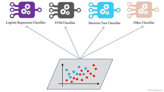
二、集成算法的基本思想

训练时用多种分类器一起完成同一任务：

测试时，对待测样本分别选取不同分类器进行，然后再汇总最后的结果：

---

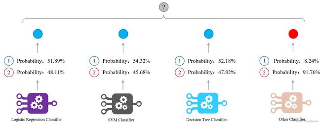
三、集成算法的简单实现：硬投票与软投票

• 硬投票：将每个分类器的结果汇总，以类似于少数服从多数的策略
• 软投票：将各分类器的结果进行加权平均（要求各分类器能得到概率值）

1、构建测试数据集

# 导入切分数据集的库
from sklearn.model_selection import train_test_split

# 导入“双月牙”数据集库
from sklearn.datasets import make_moons

# 构建测试数据
X, y = make_moons(n_samples = 500, noise = 0.3, random_state = 43)

# 划分训练集与测试集
X_train, X_test,y_train, y_test = train_test_split(X, y ,random_state = 43)

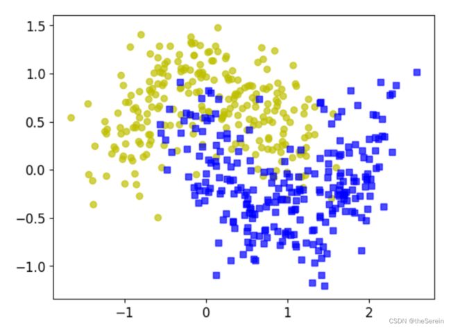
# 画图展示构建的数据集
plt.plot(X[:,0][y==0],X[:,1][y==0],'yo', alpha = 0.7)
plt.plot(X[:,0][y==1],X[:,1][y==1],'bs', alpha = 0.7)

[Out]

2、硬投票

# 导入分类器模型以及一个投票器
from sklearn.ensemble import RandomForestClassifier,VotingClassifier
from sklearn.linear_model import LogisticRegression
from sklearn.svm import SVC

# 创建三个不同的分类器
log_clf = LogisticRegression(random_state = 6)
rnd_clf = RandomForestClassifier(random_state = 6)
svm_clf = SVC(random_state = 6)

# 将三个分类器放入投票器中，并指定投票方式：Hard or Soft
# 此时，就可以视 voting_clf 为一个集成模型
voting_clf = VotingClassifier(estimators =[('lr', log_clf),('rf' ,rnd_clf), ('svc' , svm_clf)], voting='hard')

# 导入用于评估分类问题的库
from sklearn.metrics import accuracy_score

# 分别查看各分类器以及构建的集成模型的得分
for clf in (log_clf, rnd_clf, svm_clf, voting_clf):
    
    # 训练模型
    clf.fit(X_train, y_train)
    
    # 测试模型
    y_pred = clf.predict(X_test)
    
    # 查看预测结果
    print("分类器 {} 得分为：{}".format(clf.__class__.__name__, accuracy_score(y_test, y_pred)))

[Out]
	分类器 LogisticRegression 得分为：0.864
	分类器 RandomForestClassifier 得分为：0.896
	分类器 SVC 得分为：0.92
	分类器 VotingClassifier 得分为：0.912

结果说明：硬投票以牺牲时间为代价企图换取更好的分类效果，但在这个例子中，其提升并不是特别大（甚至相较 SVM 还略有下降）。

3、软投票

# 导入分类器模型以及一个投票器
from sklearn.ensemble import RandomForestClassifier,VotingClassifier
from sklearn.linear_model import LogisticRegression
from sklearn.svm import SVC

# 创建三个不同的分类器
log_clf = LogisticRegression(random_state = 6)
rnd_clf = RandomForestClassifier(random_state = 6)
# 软投票要求每个分类器都能给出概率值，因此这里必须让 SVM 返回一个概率，需调整一下参数
svm_clf = SVC(probability = True, random_state = 6)

# 将三个分类器放入投票器中，并指定投票方式：Hard or Soft
# 此时，就可以视 voting_clf 为一个集成模型
voting_clf = VotingClassifier(estimators =[('lr', log_clf),('rf' ,rnd_clf), ('svc' , svm_clf)], voting='soft')

# 导入用于评估分类问题的库
from sklearn.metrics import accuracy_score

# 分别查看各分类器以及构建的集成模型的得分
for clf in (log_clf, rnd_clf, svm_clf, voting_clf):
    
    # 训练模型
    clf.fit(X_train, y_train)
    
    # 测试模型
    y_pred = clf.predict(X_test)
    
    # 查看预测结果
    print("分类器 {} 得分为：{}".format(clf.__class__.__name__, accuracy_score(y_test, y_pred)))

[Out]
	分类器 LogisticRegression 得分为：0.864
	分类器 RandomForestClassifier 得分为：0.896
	分类器 SVC 得分为：0.92
	分类器 VotingClassifier 得分为：0.896

结果说明：从理论上说，软投票取得的效果应该要比硬投票更好，但在这个例子中，软投票策略并没有展现出它的优势。

---

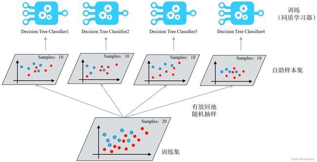
四、集成学习：Bagging 模型

• 首先对训练数据集进行多次采样，保证每次得到的采样数据都是不同的。
• 分别训练多个同质模型，例如树模型。
• 预测时需得到所有模型的预测结果再进行集成。

1、实验：对比 Bagging 模型与传统算法的差异

# 引入 Bagging 分类器的库
from sklearn.ensemble import BaggingClassifier

# 引入决策树的库
from sklearn.tree import DecisionTreeClassifier

# 构建 Bagging 分类器
# 参数一：以决策树作为基学习器
# 参数二：基学习器的数量
# 参数三：单个基学习器最多传入多少样本
# 参数四：对样本数据是否进行有放回的采样
# 参数五：是否进行多线程（设置参数为 -1 表示启用全部 GPU）
bag_clf = BaggingClassifier(DecisionTreeClassifier(),
                  n_estimators = 500,
                  max_samples = 100,
                  bootstrap = True,
                  n_jobs = -1,
                random_state = 42
)

# 训练分类器
bag_clf.fit(X_train, y_train)

# 执行预测
y_pred = bag_clf.predict(X_test)

# 查看分类效果
accuracy_score(y_test,y_pred)

[Out]
	0.912

# 定义一个树模型（用于对比）
tree_clf = DecisionTreeClassifier(random_state = 42)

# 训练模型
tree_clf.fit(X_train, y_train)

# 执行预测
y_pred_tree = tree_clf.predict(X_test)

# 查看分类效果
accuracy_score(y_test, y_pred_tree)

[Out]
	0.872

结果说明：以上结果表明，集成算法相较于单个基学习器（传统算法）而言，其提升效果还是很不错的。

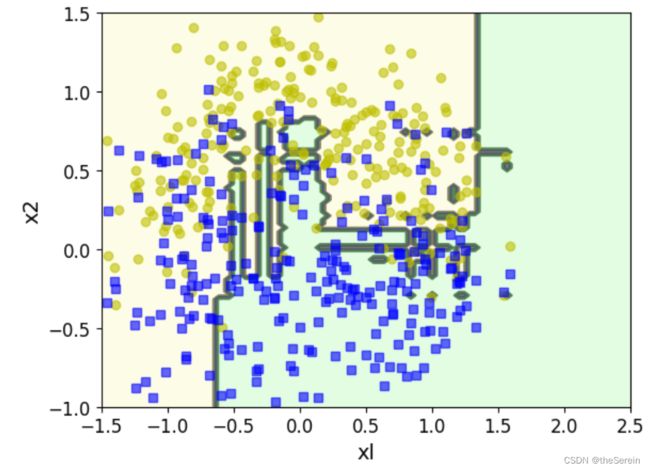
下面以可视化的方式（绘制决策边界）展示 Bagging 与传统算法的差异：

# 导入与颜色相关的库
from matplotlib.colors import ListedColormap

# 参数一：分类器
# 参数二：数据集（特征值 X）
# 参数三：数据集（标签值 y）
# 参数四：绘制的图像取值范围
# 参数五：透明程度
# 参数六：是否展示轮廓并进行填充
def plot_decision_boundary(clf, X, y, axes = [-1.5, 2.5, -1, 1.5], alpha = 0.5, contour = True):
    
    # 构建棋盘数据
    x1s=np.linspace (axes[0], axes[1],100)
    x2s=np.linspace (axes[2], axes[3],100)
    x1,x2 = np.meshgrid(x1s,x2s)
    X_new = np.c_[x1.ravel(), x2.ravel()]
    
    # 得到对指定特征的预测值
    y_pred = clf.predict(X_new).reshape(x1.shape)
    
    # 构建轮廓参数
    custom_cmap = ListedColormap(['#fafab0', '#9898ff', '#a0faa0'])
    plt.contourf(x1,x2,y_pred,cmap = custom_cmap,alpha = 0.3)
    
    # 判断是否展示轮廓
    if contour :
        custom_cmap2 = ListedColormap(['#7d7d58','#4c4c7f', '#507d50'])
        plt.contour(x1,x2,y_pred, cmap = custom_cmap2, alpha=0.8)
        plt.plot(X[:, 0][y==0],X[:,1][y==0], 'yo', alpha = 0.6)
        
    # 绘制原始数据
    plt.plot(X[:,0][y==0],X[:,1][y==1], 'bs',alpha = 0.6)
    plt.axis(axes)
    plt.xlabel('x1')
    plt.ylabel('x2')

备注： 对于颜色参数的设置，可参考此博客：https://blog.csdn.net/zhaogeng111/article/details/78419015

# 绘图展示
plt.figure(figsize = (12,5))
plt. subplot(121)
plot_decision_boundary (tree_clf,X, y)
plt.title('Decision Tree')
plt.subplot(122)
plot_decision_boundary (bag_clf,X, y)
plt.title('Decision Tree With Bagging')

结果说明： 上图中，决策树绘制出的决策边界很复杂，表示其出现了一定程度的过拟合现象；而 Bagging 模型绘制的决策边界更简单、平稳，表示其拟合效果也更好。

2、OOB 策略（out of bag）

在 Bagging 方法中， Bootstrap 每次都有一定比例的样本不会出现在其所采集的样本集合中，当然也就没有参加决策树的建立，此时，可以考虑将这部分数据用于取代测试集进行测试，而这部分数据就被称为袋外数据 OOB (Out of Bag)。

# 构建 Bagging 分类器（将 oob_score 参数置为 True）
bag_clf = BaggingClassifier(DecisionTreeClassifier(),
                  n_estimators =500,
                  max_samples = 100,
                  bootstrap = True,
                  n_jobs = -1,
                  random_state = 42,
                  oob_score = True
)

# 训练分类器
bag_clf.fit(X_train, y_train)

#  查看基于包外数据进行测试而得到的得分
bag_clf.oob_score_

[Out]
	0.8933333333333333

# 利用训练好的分类器对测试数据进行预测
y_pred = bag_clf.predict(X_test)

# 查看基于测试数据而得到的得分
accuracy_score(y_test,y_pred)

[Out]
	0.912

# 可以通过 oob_decision_function_ 属性来查看每个数据属于各分类的概率值
bag_clf.oob_decision_function_

3、随机森林（Random Forest）

随机森林是Bagging算法的典型代表，它有一个很重要的属性是可以查看数据集的“特征重要性”，下面将通过 iris 数据集对此进行实验。

# 导入随机森林的库
from sklearn. ensemble import RandomForestClassifier

# 导入鸢尾花数据集
from sklearn.datasets import load_iris

# 加载数据集
iris = load_iris()

# 建立一个基于随机森林的分类器
rf_clf = RandomForestClassifier(n_estimators=500,n_jobs=-1)

# 训练数据
rf_clf.fit(iris['data'],iris['target'])

# 查看各个特征的重要性程度
for name, score in zip(iris['feature_names'],rf_clf.feature_importances_):
    print(name, score)

[Out]
	sepal length (cm) 0.10786529772603491
	sepal width (cm) 0.026114910898121808
	petal length (cm) 0.44377248611730075
	petal width (cm) 0.42224730525854254

上面显示了各特征其重要程度的绝对占比（总和为 1），可以看出，在鸢尾花数据集中，特征：petal length 和 petal width 是相对重要的。

为了更清楚地查看各特征的影响因子，下面通过热度图来展示 Mnist 数据集中，比较重要的特征（像素点）。

# 手写数据集 Mnist 的导入有问题
# from sklearn.datasets import fetch_openml
# mnist = fetch_openml('MNIST original')

# from sklearn.datasets import fetch_openml
# mnist = fetch_openml('mnist_784')
# x = mnist.data
# y = mnist.target

# 导入本地下载好的 Mnist 数据（该数据集中，每个图片的规格为 28 × 28 = 784）
import scipy.io
mnist = scipy.io.loadmat('./resources/mnist-original.mat')

# 建立一个基于随机森林的分类器
rf_clf = RandomForestClassifier(n_estimators=500,n_jobs=-1)

# 训练分类器
rf_clf.fit(mnist['data'].T,mnist['label'].T)

# 查看 Mnist 数据集的 feature_importances_ 规格
rf_clf.feature_importances_.shape

[Out]
	(784,)

该属性反馈了 Mnist 图像数据中，每个像素点重要性的占比。接下来我们将这个数据还原为 28 × 28 的规格并基于这些数据值绘制热度图。

# 定义一个函数
def plot_digit(data):
    # 重设数据规格
    image = data.reshape (28,28)
    
    # 绘制指定数据的图像，第二个参数指定的是选择绘制热度图
    plt.imshow(image, cmap = matplotlib.cm.hot)
    
    # 去除坐标轴
    plt.axis('off')
    
# 调用定义的的函数进行图像绘制
plot_digit(rf_clf.feature_importances_)

# 绘制 colorbar（说明深色和浅色各自代表的含义）
colorbar = plt.colorbar(ticks=[rf_clf.feature_importances_.min(),rf_clf.feature_importances_.max()])

# 对前面绘制的 colorbar 进行解释
colorbar.ax.set_yticklabels(['Not important', 'Very important'])

[Out]

---

五、集成学习：Boosting 模型

1、AdaBoost 算法

上一次分类错误的数据，接下来需要重点关注（就像上学时，我们的错题本）。
即：在当前集成模型中，预测错误的观测数据的权重将增加，而预测正确的观测数据的权重则减小。

下面以 SVM 为例来演示 Adaboost 的算法流程（SVM也是一种机器学习算法，此处不知道它的细节没关系，后面会更新博客专门对其进行讲解，这里你只要知道它是一个分类器就 OK 了）：

# 导入 SVM 的库
from sklearn.svm import SVC

# 获取训练数据的规格
m = len(X_train)

# 画图展示集成策略每步做了什么工作
plt.figure(figsize=(14,5))

# 循环
for subplot,learning_rate in ((121,1),(122,0.5)):
    
    # 设置权重项：算法开始，将全部样本的权重都设为相同值
    sample_weights = np.ones(m) 
    
    # 绘制子图
    plt.subplot(subplot)
    
    # 构建 5 次模型（绘制 5 条决策边界曲线）
    for i in range(5):
        
        # 设置 SVM 分类器的核函数为 高斯核、软间隔（控制过拟合）为0.05
        svm_clf = SVC(kernel = 'rbf', C=0.05, random_state = 43)
        
        # 训练分类器
        svm_clf.fit(X_train,y_train,sample_weight = sample_weights)
        
        # 预测
        y_pred = svm_clf.predict(X_train)
        
        # 更新权重参数
        sample_weights[y_pred != y_train] *= (1+learning_rate)
        
        # 绘制决策边界
        plot_decision_boundary(svm_clf, X, y, alpha=0.2)
        
    # 绘制图像标题
    plt.title('learning_rate = {}'.format(learning_rate))
    
    # 展示每条线对应模型的第几次构建
    if subplot == 121:
        plt.text(-0.5,-0.65,"1", fontsize=15)
        plt.text(-0.6,-0.30,"2", fontsize=15)
        plt.text(-0.5,0.10,"3", fontsize=15)
        plt.text(-0.4,0.55,"4", fontsize=15)
        plt.text(-0.3,0.90,"5", fontsize=15)

其输出如下：

上面的过程演示了如何用基学习器手动实现 AdaBoost 算法，下面我们用封装好的函数直接实现：

# 接下来直接调用 AdaBoost 的库
from sklearn. ensemble import AdaBoostClassifier

# 构建基于 AdaBoost 模型的分类器
# max_depth：模型的深度
# n_estimators：模型的迭代次数
# learning_rate：学习率
ada_clf = AdaBoostClassifier(DecisionTreeClassifier(max_depth = 2),
            n_estimators = 200,
            learning_rate = 0.5,random_state = 42
)

# 训练模型
ada_clf.fit(X_train,y_train)

# 绘制决策边界
plot_decision_boundary(ada_clf,X,y)

2、Gradient Boosting 算法

把所有学习器的结果累加起来得出最终结论!

(1) Gradient Boosting 的算法流程

下面以决策回归树为例来演示 Gradient Boosting 的算法流程：

# 构建新的样本数据集
np.random.seed(42)
X = np.random.rand(100,1) - 0.5
y =3*X[:,0]**2 + 0.05*np.random.randn(100)

# 导入决策回归树的库
from sklearn.tree import DecisionTreeRegressor

# 建立第一棵决策回归树
tree_reg1 = DecisionTreeRegressor(max_depth = 2)

# 训练模型
tree_reg1.fit(X,y)

[Out]

# 接下来算出残差
y2 = y - tree_reg1.predict(X)

# 然后利用 y2 建立第二棵决策回归树
tree_reg2 = DecisionTreeRegressor(max_depth = 2)

# 训练模型
tree_reg2.fit(X, y2)

[Out]

# 继续计算残差
y3 = y2 - tree_reg2.predict(X)

# 建立第三棵决策回归树
tree_reg3 = DecisionTreeRegressor(max_depth = 2)

# 训练模型
tree_reg3.fit(X, y3)

[Out]

# 接下来构建一个测试数据
X_new = np.array([[0.25]])

# 基于前面 3 棵树模型对该测试数据进行预测
y_pred = sum(tree.predict(X_new) for tree in (tree_reg1,tree_reg2,tree_reg3))

# 查看预测结果
print("{} 对应的真实值大致为 {}，预测值为 {}".format(X_new[0],3*X_new[0]**2,y_pred))  

[Out]
	[0.25] 对应的真实值大致为 [0.1875]，预测值为 [0.17052257]

上面的实验演示了 Gradient Boosting 的工作流程，为了更直观地查看这个过程，下面对其进行可视化。

(2) 可视化展示 Gradient Boosting 流程

# 定义绘图函数
def plot_predictions(regressors,X, y, axes,label=None,style="r-",data_style="b.", data_label=None):
    
    # 定义样本数据点（X 轴）
    x1 = np.linspace(axes[0],axes[1],500)
    
    # 得到最终的预测值
    y_pred = sum(regressor.predict(x1.reshape(-1,1)) for regressor in regressors)
    
    # 绘制样本数据点
    plt.plot(X[:,0], y, data_style, label=data_label)
    
    # 绘制预测值
    plt.plot(x1,y_pred,style,linewidth=2,label=label)
    
    # 绘制图像标签
    if label or data_label:
        plt.legend(loc="upper center", fontsize=16)
        
    # 绘制图像的坐标轴
    plt.axis(axes)

# 下面进行画图展示
plt.figure(figsize=(11,11))

plt.subplot(321)
plot_predictions([tree_reg1],X, y, axes=[-0.5,0.5,-0.1,0.8],label="$h_1(x_1)$", style="g-",data_label="Training set")
plt.ylabel("$y$", fontsize=16, rotation=0)
plt.title("Residuals and tree predictions", fontsize=16)

plt.subplot(322)
plot_predictions([tree_reg1],X, y, axes=[-0.5,0.5,-0.1,0.8], label="$h(x_1) = h_1(x_1)$",data_label="Training set")
plt.ylabel ("$y$",fontsize=16, rotation=0)
plt.title("Ensemble predictions", fontsize=16)

plt.subplot(323)
plot_predictions([tree_reg2],X, y2, axes=[-0.5,0.5,-0.5,0.5],label="$h_2(x_1)$", style="g-" , data_style ="k+ ", data_label= "Residuals")
plt.ylabel("$y - h_1(x_1)$",fontsize=16)

plt.subplot(324)
plot_predictions([tree_reg1,tree_reg2],X, y, axes=[-0.5,0.5,-0.1,0.8],label="$h(x_1) = h_1(x_1) + h_2(x_1)$")
plt.ylabel("$y$", fontsize=16,rotation=0)

plt.subplot (325)
plot_predictions([tree_reg3],X, y3,axes=[-0.5,0.5,-0.5,0.5],label="$h_3(x_1)$",style="g-",data_style="k+", data_label= "Residuals")
plt.ylabel("$y - h_1(x_1) - h_2(x_1)$",fontsize=16)
plt.xlabel("$x_1$", fontsize=16)

plt.subplot(326)
plot_predictions([tree_reg1,tree_reg2,tree_reg3],X,y,axes=[-0.5,0.5,-0.1,0.8],label = "$h(x_1) = h_1(x_1) + h_2(x_1) + h_3(x_1)$")
plt.xlabel("$x_1$", fontsize=16)
plt.ylabel("$y$", fontsize=16, rotation=0)

plt.show ()

[Out]

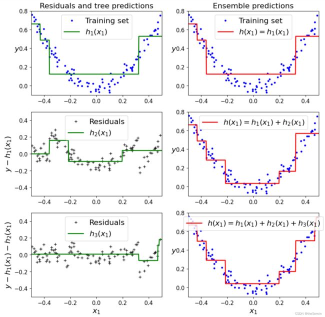
上图中，第一次拟合得到的决策树预测出的数据大致符合原始数据曲线的分布情况（图1）；而第二棵树基于第一棵树，在对残差数据进行拟合，其得到的拟合曲线也大致符合残差数据的分布情况（图3）；第三棵树基于第一、二棵树，在对残差数据进行拟合，其得到的拟合曲线也大致符合残差数据的分布情况（图5）。图 2、4、6 则分别给出了在对当前已构建决策树进行叠加后，其得到的集成模型。

现实中，有许多现成框架实现了 Gradient Boosting 的工作，需要时可以直接调用相关库。如：

• 第一代 sklearn-GBDT（不常用，过去式了）
• 第二代 Xgboost
• 第三代 lightgbm
• ……

下面选取 sklearn 中现成的 GBDT 模型进行演示

(3) 实验：练习 sklearn 中现成的 GBDT 模型

# 导入 GBDT 库
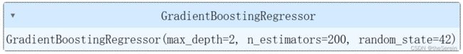
from sklearn.ensemble import GradientBoostingRegressor

# 构建一个 GBDT 模型
# max_depth：树的最大深度
# n_estimators：子树的数量
# learning_rate：学习率（这个学习率和梯度下降中的不一样，这里的学习率主要是控制每棵树的所占权重）
# 这些参数和树模型的参数类似
gbdt = GradientBoostingRegressor(max_depth = 2,
                         n_estimators = 3,
                         learning_rate = 1.0,
                         random_state = 42
                         )

# 训练模型
gbdt.fit(X,y)

[Out]

# 为了便于做对比试验，接下来再建立两个 GBDT 模型
gbdt_slow_1 = GradientBoostingRegressor(max_depth = 2,
                         n_estimators = 3,
                         learning_rate = 0.1,
                         random_state = 42
                         )

# 训练模型
gbdt_slow_1.fit(X,y)

# 构建模型
gbdt_slow_2 = GradientBoostingRegressor(max_depth = 2,
                         n_estimators = 200,
                         learning_rate = 0.1,
                         random_state = 42
                         )

# 训练模型
gbdt_slow_2.fit(X,y)

[Out]

# 对比试验 1：探究在相同迭代次数下，不同学习率的差异
plt.figure(figsize = (11,4))
plt.subplot(121)
plot_predictions([gbdt],X,y,axes=[-0.5,0.5,-0.1,0.8],label='GBDT Predictions')
plt.title('learning_rate={}, n_estimators={}'.format(gbdt.learning_rate,gbdt.n_estimators))

plt.subplot(122)
plot_predictions([gbdt_slow_1],X,y,axes=[-0.5,0.5,-0.1,0.8],label='GBDT Predictions')
plt.title('learning_rate={}, n_estimators={}'.format(gbdt_slow_1.learning_rate,gbdt_slow_1.n_estimators))

[Out]

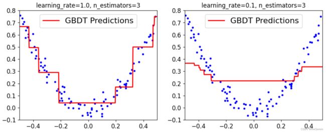
上图表明，当子树个数较小时，学习率要尽可能大才能得到较好的拟合效果。但是，在实际使用时，我们通常是让学习率偏低（防止过拟合），并设置更多的子树来提高拟合效果。

# 对比试验 2：探究在相同学习率的条件下，不同子树数量的差异
plt.figure(figsize = (11,4))
plt.subplot(121)
plot_predictions([gbdt_slow_2],X,y,axes=[-0.5,0.5,-0.1,0.8],label='GBDT Predictions')
plt.title('learning_rate={}, n_estimators={}'.format(gbdt_slow_2.learning_rate,gbdt_slow_2.n_estimators))

plt.subplot(122)
plot_predictions([gbdt_slow_1],X,y,axes=[-0.5,0.5,-0.1,0.8],label='GBDT Predictions')
plt.title('learning_rate={}, n_estimators={}'.format(gbdt_slow_1.learning_rate,gbdt_slow_1.n_estimators))

[Out]

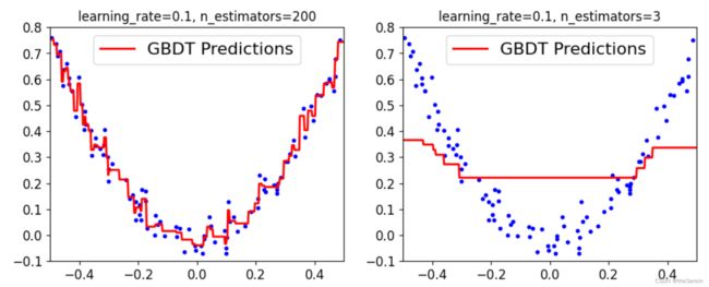
上图表明，当学习率较低时（且每棵子树的深度较小），则子树数量越多，其拟合效果越好。

(4) 提前停止策略

在 GDBT 中，随着 n_estimators（集成模型中子树数量） 的增加，损失函数的值并不一定总是严格单减；另一方面，集成模型中子树数量较多的模型也并不一定总是比子树较少的模型更具性价比（即更多的训练时间并没有换到差距足够大的训练效果）。因此，我们必须找到一个合适的时机终止算法，降低时间开销。

# 引入计算均方误差的库
from sklearn.metrics import mean_squared_error

# 切分数据集得到新的训练集和测试集
X_train,X_val,y_train,y_val = train_test_split(X, y, random_state=49)

# 构建新的 GDBT 模型
gbdt = GradientBoostingRegressor(max_depth = 2,
                         n_estimators = 120,
                         random_state = 42
                         )

# 训练数据
gbdt.fit(X_train,y_train)

# 查看模型的训练结果（这里查看的结果是分阶段的，即模型在测试数据规模为：1、2、3、…… 时的）
# 这里需要用到一个分阶段预测的函数：staged_predict
errors = [mean_squared_error(y_val,y_pred) for y_pred in gbdt.staged_predict(X_val)]

# 取出均方误差最小的的那一次（即在测试集上取得最佳效果）的子树数量
bst_n_estimators = np.argmin(errors) + 1
min_error = np.min(errors)
print("在 GBDT 模型中，当总的子树数量为 {} 时，\n取得最佳效果的子树数量为 {}，\n其在测试集上的均方误差为 {}。".format(len(errors),bst_n_estimators,min_error))

[Out]
	在 GBDT 模型中，当总的子树数量为 120 时，
	取得最佳效果的子树数量为 56，
	其在测试集上的均方误差为 0.002712853325235463。

# 接下来绘图展示最佳子树数量的 GBDT 模型的拟合效果
# 构建最佳子树数量的 GBDT 模型（控制其他参数不变）
gbdt_best = GradientBoostingRegressor(max_depth = 2,
                         n_estimators = bst_n_estimators,
                         random_state = 42
                         )

# 训练新模型
gbdt_best.fit(X_train, y_train)

# 绘图展示
# 设置图像规格
plt.figure(figsize = (11,4))

plt.subplot(121)

# 绘制原始 GBDT 模型分阶段的均方误差
plt.plot(errors,'b-')

# 绘制最佳子树数量的虚线
plt.plot([bst_n_estimators,bst_n_estimators],[0,min_error],'k--')
plt.plot([0,120],[min_error,min_error],'k--')
plt.axis([0,120,0,0.01])
plt.title('Val Error')

# 绘制最佳 GBDT 模型的拟合情况
plt.subplot(122)
plot_predictions([gbdt_best],X,y,axes=[-0.5,0.5,-0.1,0.8])
plt.title('Best Model(%d trees)'%bst_n_estimators)

[Out]

如何实现提前停止？

一种比较直观的方式就是上面演示的那样：训练全部子树，最后分阶段统计出在测试集合上均方误差最小的子树数量，然后再以该数量为 n_estimators 参数训练模型。但是，这样的方式本质上还是训练了全部数量的子树。最好的办法是：每次训练仅训练一棵子树，接下来统计出该 GBDT 模型在测试集上的效果；当下一次训练时，依然仅训练一棵子树，然后将该子树加入之前已经构建好的集成模型中再进行测试。这样叠加式的训练其实只需要在构建 GBDT 模型时加入一个热启动参数 warm_start 即可：

# 通过 “热启动” 参数实现提前停止
gbdt_auto = GradientBoostingRegressor(max_depth = 2,
                         # 打开热启动参数（此时，就不需要 n_estimators 参数了，而是在循环中自行寻找并动态调整）
                         warm_start = True,
                         random_state = 42
                         )

# 最大上浮次数
MAX_FLAW = 5

# 当前上浮次数
error_going_up = 0

# 设置用于记录“在验证集上取到的最小均方误差”，初始值要足够大
min_val_error = float('inf')

# 设置取得最小均方误差时的 n_estimators 值
min_val_error_estimators = 0

# 循环查找最佳子树数量
for n_estimators in range(1,120):
    
    # 动态设置 GBDT 模型的 n_estimators 参数
    gbdt_auto.n_estimators = n_estimators
    
    # 训练模型
    gbdt_auto.fit(X_train,y_train)
    
    # 对验证集进行预测
    y_pred = gbdt_auto.predict(X_val)
    
    # 计算在验证集上的均方误差
    val_error = mean_squared_error(y_val, y_pred)
    
    # 如果该误差值低于指定值则记录下该值
    if val_error < min_val_error:
        min_val_error = val_error
        min_val_error_estimators = n_estimators
        error_going_up = 0
        
    # 否则说明：此次新加入一棵子树，反而使得整个集成模型的预测能力降低
    # 这种情况暗示接下来继续加入新的子树是在“梯度上升”
    # 此时，我们可以对这种情况进行统计（并规定：当上升次数超过最大上浮次数 MAX_FLAW 时就退出循环）    
    else:
        error_going_up += 1
        if(error_going_up == MAX_FLAW):
            break

# 输出最终得到的最佳子树数量 n_estimators
print("在验证集上取得最小均方误差时，子树数量为 {}，均方误差为 {}。".format(min_val_error_estimators,min_val_error))

[Out]
	在验证集上取得最小均方误差时，子树数量为 56，均方误差为 0.002712853325235463。

---

六、集成学习：Stacking 模型

Stacking 策略在预测时主要有两个阶段：

• 将原始数据集分别交给 L 个异质弱学习器进行预测；
• 将 L 个异质弱学习器的预测结果作为输入再交给一个元模型进行汇总，并由该元模型输出最终结果。

阶段一：训练异质学习器

# 导入用于加载本地资源的库
import scipy.io

# 加载本地 Mnist 数据集（十分类任务）
# 没有该数据集的小伙伴可以去此专栏下 “ 【机器学习】Sklearn导入手写数字数据集 Mnist 失败的解决办法 ” 中下载
mnist = scipy.io.loadmat('./resources/mnist-original.mat')

# 划分训练集与验证集
X_train,X_val, y_train,y_val = train_test_split (
    mnist['data'].T,mnist['label'].T,test_size=10000,random_state=42)

# 选择几种不同的分类器（导入库）
from sklearn.ensemble import RandomForestClassifier,ExtraTreesClassifier
from sklearn.svm import LinearSVC
from sklearn.neural_network import MLPClassifier

# 构建异质弱学习器
random_forest_clf = RandomForestClassifier(random_state = 42)
extra_trees_clf = ExtraTreesClassifier(random_state = 42)
svm_clf = LinearSVC(random_state = 42)
mlp_clf = MLPClassifier(random_state = 42)

# 将异质弱学习器加入一个列表
estimators = [random_forest_clf,extra_trees_clf,svm_clf,mlp_clf]

# 接下来分别训练这些分类器
for estimator in estimators:
    print("Training the", estimator)
    estimator.fit(X_train, y_train)

[Out]
	Training the RandomForestClassifier(random_state=42)
	Training the ExtraTreesClassifier(random_state=42)
	Training the LinearSVC(random_state=42)
	Training the MLPClassifier(random_state=42)

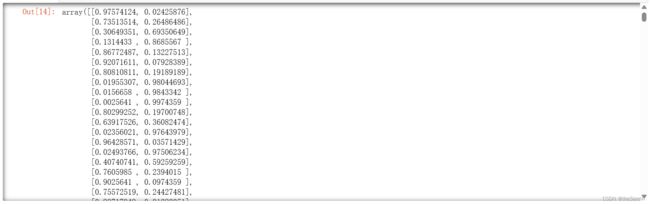
阶段二：用异质学习器的预测结果作为输入，训练组合它们的元模型

# 设置用于存放“不同学习器的预测结果”的数组
X_val_predictions = np.empty((len(X_val),len(estimators)), dtype=np.float32)

# 获取不同学习器的预测结果（基于验证集，这里一定要用与前面训练阶段不同的数据集）
for index,estimator in enumerate(estimators):
    X_val_predictions[:,index] = estimator.predict(X_val)
    
# 查看不同学习器的预测结果
X_val_predictions

[Out]
	array([[7., 7., 7., 7.],
	       [8., 8., 8., 8.],
	       [6., 6., 6., 6.],
	       ...,
	       [9., 9., 9., 9.],
	       [1., 1., 1., 1.],
	       [6., 6., 6., 6.]], dtype=float32)

# 构建用于组合异质学习器预测结果的元模型（这里选择的是随机森林）
rnd_forest_blender = RandomForestClassifier(n_estimators=200, oob_score=True,random_state=42)

# 基于对验证集的预测结果（另一组数据），训练用于汇总的元模型
rnd_forest_blender.fit(X_val_predictions,y_val)

# 查看 OOB 指标
rnd_forest_blender.oob_score_

[Out]
	0.9701

END

---