PyTorch LSTM和LSTMP的原理及其手写复现
PyTorch LSTM和LSTMP的原理及其手写复现
- 0、前言
- 全部参数的细致介绍
- 代码实现
- Reference
0、前言
关于LSTM的原理以及公式其实在这篇博客一步一步详解LSTM网络【从RNN到LSTM到GRU等,直至attention】讲的非常清晰明了了。
这里就是写出LSTM的pytorch的实现,包括API和手写。
在看代码之前有必要了解输入输出有哪些,以及他们的特性。
官方教程在:
https://pytorch.org/docs/stable/generated/torch.nn.LSTM.html#torch.nn.LSTM


全部参数的细致介绍
将多层长短期记忆 (LSTM) RNN 应用于输入序列。
对于输入序列中的每个元素,每一层计算以下函数:
i t = σ ( W i i x t + b i i + W h i h t − 1 + b h i ) f t = σ ( W i f x t + b i f + W h f h t − 1 + b h f ) g t = tanh ( W i g x t + b i g + W h g h t − 1 + b h g ) o t = σ ( W i o x t + b i o + W h o h t − 1 + b h o ) c t = f t ⊙ c t − 1 + i t ⊙ g t h t = o t ⊙ tanh ( c t ) \begin{align} i_t &= \sigma(W_{ii} x_t + b_{ii} + W_{hi} h_{t-1} + b_{hi}) \\ f_t &= \sigma(W_{if} x_t + b_{if} + W_{hf} h_{t-1} + b_{hf}) \\ g_t &= \tanh(W_{ig} x_t + b_{ig} + W_{hg} h_{t-1} + b_{hg}) \\ o_t &= \sigma(W_{io} x_t + b_{io} + W_{ho} h_{t-1} + b_{ho}) \\ c_t &= f_t \odot c_{t-1} + i_t \odot g_t \\ h_t &= o_t \odot \tanh(c_t) \end{align} itftgtotctht=σ(Wiixt+bii+Whiht−1+bhi)=σ(Wifxt+bif+Whfht−1+bhf)=tanh(Wigxt+big+Whght−1+bhg)=σ(Wioxt+bio+Whoht−1+bho)=ft⊙ct−1+it⊙gt=ot⊙tanh(ct)
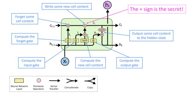
其中 h t h_t ht是时间t的隐藏状态, c t c_t ct是时间t的cell状态, x t x_t xt是时间t的输入, h t − 1 h_{t-1} ht−1是层的隐藏状态在时间 t-1 或时间 0 的初始隐藏状态,而 i t i_t it、 f t f_t ft、 g t g_t gt、 o t o_t ot 分别是输入门、遗忘门、单元门和输出门。 σ \sigma σ是sigmoid函数, ⊙ \odot ⊙是Hadamard积。( g t g_t gt也可称为New cell content)
遗忘门控制遗忘 c t − 1 c_{t-1} ct−1的多少即 f t ⊙ c t − 1 f_t \odot c_{t-1} ft⊙ct−1,而输出门是控制输出New cell content的多少即 i t ⊙ g t i_t \odot g_t it⊙gt,若 f t f_t ft=1且 i t i_t it=0则细胞状态一直保存下去。
输出门是控制输出多少当前细胞状态,即 o t ⊙ tanh ( c t ) o_t \odot \tanh(c_t) ot⊙tanh(ct)。
在多层LSTM中,第l层(l >= 2)的输入 x t ( l ) x^{(l)}_t xt(l)是前一层的隐藏状态 h t ( l − 1 ) h^{(l-1)}_t ht(l−1) 乘以 dropout δ t ( l − 1 ) \delta^{(l-1)}_t δt(l−1) 其中每个 δ t ( l − 1 ) \delta^{(l- 1)}_t δt(l−1) 是一个伯努利随机变量,which is 0 with probabilitydropout。
如果指定 proj_size > 0,将使用带投影的 LSTM。这会以下列方式更改 LSTM 单元。
首先, h t h_t ht 的维度将从hidden_size更改为proj_size( W h i W_{hi} Whi 的维度将相应更改)。
其次,每一层的输出隐藏状态将乘以一个可学习的投影矩阵: h t = W h r h t h_t = W_{hr}h_t ht=Whrht。
请注意,因此,LSTM 网络的输出也将具有不同的形状。
有关所有变量的确切维度,请参阅下面的输入/输出部分。您可以在 https://arxiv.org/abs/1402.1128 中找到更多详细信息。
参数:
input_size– 输入 x 中预期特征的数量hidden_size– 隐藏状态h的特征数num_layers– 循环层数。例如,设置num_layers=2意味着将两个 LSTM 堆叠在一起形成一个堆叠 LSTM,第二个 LSTM 接收第一个 LSTM 的输出并计算最终结果。默认值:1bias– 如果为False,则该层不使用偏置权重 b i h b_{ih} bih 和 b h h b_{hh} bhh。默认值:Truebatch_first– 如果为True,则输入和输出张量将作为 (batch, seq, feature) 而不是 (seq, batch, feature) 提供。请注意,这不适用于隐藏状态或细胞状态。有关详细信息,请参阅下面的输入/输出部分。默认值:Falsedropout– 如果非零,则在除最后一层之外的每个 RNN 层的输出上引入一个 Dropout 层,dropout 概率等于dropout。默认值:0bidirectional– 如果为True,则成为双向 LSTM。默认值:Falseproj_size– 如果> 0,将使用具有相应大小投影的 LSTM。默认值:0
(相比于RNN只是多了一个proj_size)
输入:input, (h_0, c_0)
input:对于非批处理输入,形状为 ( L , H i n ) (L, H_{in}) (L,Hin) 的张量, ( L , N , H i n ) (L, N, H_{in}) (L,N,Hin)当batch_first=False或 ( N , L , H i n ) ( N, L, H_{in}) (N,L,Hin) 当batch_first=True时包含输入序列的特征。输入也可以是打包的可变长度序列。有关详细信息,请参阅torch.nn.utils.rnn.pack_padded_sequence()或torch.nn.utils.rnn.pack_sequence()。h_0:形状张量 ( D ∗ num_layers , H o u t ) (D * \text{num\_layers}, H_{out}) (D∗num_layers,Hout) 对于非批处理输入或 ( D ∗ num_layers , N , H o u t ) (D * \text{num\_layers}, N, H_{out}) (D∗num_layers,N,Hout)包含输入序列中每个元素的初始隐藏状态。如果未提供 (h_0, c_0),则默认为零。。c_0:形状张量 ( D ∗ num_layers , H c e l l ) (D * \text{num\_layers}, H_{cell}) (D∗num_layers,Hcell)对于非批处理输入或 ( D ∗ num_layers , N , H c e l l ) ( D * \text{num\_layers}, N, H_{cell}) (D∗num_layers,N,Hcell) 包含输入序列中每个元素的初始单元状态。如果未提供 (h_0, c_0),则默认为零。
其中:
N = b a t c h s i z e L = s e q u e n c e l e n g t h D = 2 i f b i d i r e c t i o n a l = T r u e o t h e r w i s e 1 H i n = i n p u t _ s i z e H c e l l = h i d d e n _ s i z e H o u t = proj_size if proj_size > 0 otherwise hidden_size \begin{array}{l} N=batch\ size\\ L=sequence\ length\\ D=2\ if\ bidirectional=True\ otherwise\ 1\\ H_{in}=input\_size\\ H_{cell}=hidden\_size\\ H_{out} ={} \text{proj\_size if } \text{proj\_size}>0 \text{ otherwise hidden\_size} \end{array} N=batch sizeL=sequence lengthD=2 if bidirectional=True otherwise 1Hin=input_sizeHcell=hidden_sizeHout=proj_size if proj_size>0 otherwise hidden_size
尤其要注意参数的维度。
输出: output, (h_n, c_n)
output:形状张量 ( L , D ∗ H o u t ) (L, D * H_{out}) (L,D∗Hout) 对于非批处理输入, ( L , N , D ∗ H o u t ) (L, N, D * H_{out} ) (L,N,D∗Hout) 当batch_first=False或 ( N , L , D ∗ H o u t ) (N, L, D * H_{out}) (N,L,D∗Hout) 当batch_first=True对于每个 t,包含来自 LSTM 最后一层的输出特征 (h_t)。如果torch.nn.utils.rnn.PackedSequence已作为输入给出,输出也将是一个打包序列。当bidirectional=True时,输出将包含序列中每个时间步的正向和反向隐藏状态的串联。h_n:形状张量 ( D ∗ n u m _ l a y e r s , H o u t ) (D * num\_layers, H_{out}) (D∗num_layers,Hout) 对于非批处理输入或 ( D ∗ n u m _ l a y e r s , N , H o u t ) (D∗num\_layers,N,Hout) (D∗num_layers,N,Hout)包含序列中每个元素的最终隐藏状态。当bidirectional=True时,h_n 将分别包含最终前向和反向隐藏状态的串联。(其实output的最后一个元素就是h_n)c_n:形状张量 ( D ∗ num_layers , H c e l l ) (D * \text{num\_layers}, H_{cell}) (D∗num_layers,Hcell) 对于非批处理输入或 ( D ∗ num_layers , N , H c e l l ) ( D * \text{num\_layers}, N, H_{cell}) (D∗num_layers,N,Hcell) 包含序列中每个元素的最终单元状态。当bidirectional=True时,c_n 将分别包含最终正向和反向单元格状态的串联。
变量:
weight_ih_l[k]– 第 k t h \text{k}^{th} kth层 (W_ii|W_if|W_ig|W_io) 的可学习输入隐藏input-hidden权重,形状为 (4*hidden_size, input _size) 对于 k = 0。否则,形状为 (4*hidden_size, num_directions * hidden_size)。如果指定了proj_size > 0,对于 k > 0,形状将为 (4*hidden_size, num_directions * proj_size)weight_hh_l[k]– 第 k t h \text{k}^{th} kth 层 (W_hi|W_hf|W_hg|W_ho) 的可学习隐藏-隐藏hidden-hidden权重,形状为 (4*hidden_size, hidden_size)。如果指定了proj_size > 0,则形状将为 (4*hidden_size, proj_size)。bias_ih_l[k]– 第 k层 (b_ii|b_if|b_ig|b_io) 的可学习输入隐藏偏差,形状为 (4*hidden_size)bias_hh_l[k]– 第 k层 (b_hi|b_hf|b_hg|b_ho) 的可学习隐藏-隐藏偏差,形状为 (4*hidden_size)weight_hr_l[k]– 第 k层形状的可学习投影权重 (proj_size, hidden_size)。仅在指定proj_size > 0时出现。weight_ih_l[k]_reverse– 类似于反向的 weight_ih_l[k]。仅在bidirectional=True时出现。weight_hh_l[k]_reverse– 类似于反向的 weight_hh_l[k]。仅在bidirectional=True时出现。bias_ih_l[k]_reverse– 类似于反方向的 bias_ih_l[k]。仅在bidirectional=True时出现。bias_hh_l[k]_reverse– 类似于反方向的 bias_hh_l[k]。仅在bidirectional=True时出现。weight_hr_l[k]_reverse– 类似于反向的 weight_hr_l[k]。仅在指定bidirectional=True和proj_size > 0时出现。
需要注意的是:
- 所有的权重和偏置都从 U ( − k , k ) \mathcal{U}(-\sqrt{k}, \sqrt{k}) U(−k,k) 初始化,其中 k = 1 h i d d e n _ s i z e k = \frac{1 }{hidden\_size} k=hidden_size1
- 对于双向 LSTM,前向和后向分别是方向 0 和 1。
batch_first=False时分割输出层的示例:output.view(seq_len, batch, num_directions, hidden_size)。 batch_first参数对于未批处理的输入会被忽略。- 对于双向 LSTM,h_n 不等于输出的最后一个元素;前者(h_n)包含最终的正向和反向隐藏状态,而后者(outpuy)包含最终的正向隐藏状态和初始反向隐藏状态。
代码实现
LSTM API
首先实例化一些参数:
import torch
import torch.nn as nn

# 定义一些常量
batch_size, seq_len, input_size, h_size = 2, 3, 4, 5
input = torch.randn(batch_size, seq_len, input_size)  # 随机初始化一个输入序列
c_0 = torch.randn(batch_size, h_size)  # 初始值,不会参与训练
h_0 = torch.randn(batch_size, h_size)
调用PyTorch中的 LSTM API:
# 调用官方 LSTM API
lstm_layer = nn.LSTM(input_size, h_size, batch_first=True)  # num_layers默认为1
output, (h_n, c_n) = lstm_layer(input, (h_0.unsqueeze(0), c_0.unsqueeze(0)))  # (D*num_layers=1, b, hidden_size)
看一下返回的结果的形状:
print(output.shape)  # [2,3,5] [b, seq_len, hidden_size]
print(h_n.shape)  # [1,2,5] [num_layers, b, hidden_size]
print(c_n.shape)  # [1,2,5] [num_layers, b, hidden_size]
这里输出一下lstm_layer中的参数名称及其形状:
for name, para in lstm_layer.named_parameters():
    print(name, para.shape)
输出结果如下:
weight_ih_l0 torch.Size([20, 4])  # [4*hidden_size, input_size]
weight_hh_l0 torch.Size([20, 5])  # [4*hidden_size, hidden_size]
bias_ih_l0 torch.Size([20])  # [4*hidden_size]
bias_hh_l0 torch.Size([20])  # [4*hidden_size]
手写 lstm_forward 函数
这里先将lstm_forward函数中的每个参数的维度写出来:
def lstm_forward(input, initial_states, w_ih, w_hh, b_ih, b_hh):
    h_0, c_0 = initial_states  # 初始状态  [b_size, hidden_size]
    b_size, seq_len, input_size = input.shape
    h_size = h_0.shape[-1]

    h_prev, c_prev = h_0, c_0
    # 需要将权重w在batch_size维进行扩维并复制,才能和x与h进行相乘
    w_ih_batch = w_ih.unsqueeze(0).tile(b_size, 1, 1)  # [4*hidden_size, in_size]->[b_size, ,]
    w_hh_batch = w_hh.unsqueeze(0).tile(b_size, 1, 1)  # [4*hidden_size, hidden_size]->[b_size, ,]

    output_size = h_size
    output = torch.zeros(b_size, seq_len, output_size)  # 初始化一个输出序列
    for t in range(seq_len):
        x = input[:, t, :]  # 当前时刻的输入向量 [b,in_size]->[b,in_size,1]
        w_times_x = torch.bmm(w_ih_batch, x.unsqueeze(-1)).squeeze(-1)   # bmm:含有批量大小的矩阵相乘
        # [b, 4*hidden_size, 1]->[b, 4*hidden_size]
        # 这一步就是计算了 Wii*xt|Wif*xt|Wig*xt|Wio*xt
        w_times_h_prev = torch.bmm(w_hh_batch, h_prev.unsqueeze(-1)).squeeze(-1)
        # [b, 4*hidden_size, hidden_size]*[b, hidden_size, 1]->[b,4*hidden_size, 1]->[b, 4*hidden_size]
        # 这一步就是计算了 Whi*ht-1|Whf*ht-1|Whg*ht-1|Who*ht-1

        # 分别计算输入门(i)、遗忘门(f)、cell门(g)、输出门(o)  维度均为 [b, h_size]
        i_t = torch.sigmoid(w_times_x[:, :h_size] + w_times_h_prev[:, :h_size] + b_ih[:h_size] + b_hh[:h_size])  # 取前四分之一
        f_t = torch.sigmoid(w_times_x[:, h_size:2*h_size] + w_times_h_prev[:, h_size:2*h_size]
                            + b_ih[h_size:2*h_size] + b_hh[h_size:2*h_size])
        g_t = torch.tanh(w_times_x[:, 2*h_size:3*h_size] + w_times_h_prev[:, 2*h_size:3*h_size]
                         + b_ih[2*h_size:3*h_size] + b_hh[2*h_size:3*h_size])
        o_t = torch.sigmoid(w_times_x[:, 3*h_size:] + w_times_h_prev[:, 3*h_size:]
                            + b_ih[3*h_size:] + b_hh[3*h_size:])
        c_prev = f_t * c_prev + i_t * g_t
        h_prev = o_t * torch.tanh(c_prev)

        output[:, t, :] = h_prev

    return output, (h_prev.unsqueeze(0), c_prev.unsqueeze(0))  # 官方是三维,在第0维扩一维
验证一下 lstm_forward 的准确性:
# 这里使用 lstm_layer 中的参数
# 加了me表示自己手写的
output_me, (h_n_me, c_n_me) = lstm_forward(input, (h_0, c_0), lstm_layer.weight_ih_l0,
                                           lstm_layer.weight_hh_l0, lstm_layer.bias_ih_l0, lstm_layer.bias_hh_l0)
打印一下,看两个的计算结果是否相同:
print("PyTorch API output:")
print(output)  # [2,3,5] [b, seq_len, hidden_size]
print(h_n)  # [1,2,5] [num_layers, b, hidden_size]
print(c_n)  # [1,2,5] [num_layers, b, hidden_size]
print("\nlstm_forward function output:")
print(output_me)  # [2,3,5] [b, seq_len, hidden_size]
print(h_n_me)  # [1,2,5] [num_layers, b, hidden_size]
print(c_n_me)
结果如下,完全一致,说明手写的是对的:
PyTorch API output:
tensor([[[ 0.1671,  0.2493,  0.2603, -0.1448, -0.1951],
         [-0.0680,  0.0478,  0.0218,  0.0735, -0.0604],
         [ 0.0144,  0.0507, -0.0556, -0.2600,  0.1234]],

        [[ 0.4561, -0.0015, -0.0776, -0.0644, -0.5319],
         [ 0.1667,  0.0111,  0.0114, -0.1227, -0.2369],
         [-0.0220,  0.0637, -0.2353,  0.0404, -0.1309]]],
       grad_fn=<TransposeBackward0>)
tensor([[[ 0.0144,  0.0507, -0.0556, -0.2600,  0.1234],
         [-0.0220,  0.0637, -0.2353,  0.0404, -0.1309]]],
       grad_fn=<StackBackward0>)
tensor([[[ 0.0223,  0.1574, -0.1572, -0.4663,  0.2110],
         [-0.0382,  0.6440, -0.4334,  0.0779, -0.3198]]],
       grad_fn=<StackBackward0>)

lstm_forward function output:
tensor([[[ 0.1671,  0.2493,  0.2603, -0.1448, -0.1951],
         [-0.0680,  0.0478,  0.0218,  0.0735, -0.0604],
         [ 0.0144,  0.0507, -0.0556, -0.2600,  0.1234]],

        [[ 0.4561, -0.0015, -0.0776, -0.0644, -0.5319],
         [ 0.1667,  0.0111,  0.0114, -0.1227, -0.2369],
         [-0.0220,  0.0637, -0.2353,  0.0404, -0.1309]]], grad_fn=<CopySlices>)
tensor([[[ 0.0144,  0.0507, -0.0556, -0.2600,  0.1234],
         [-0.0220,  0.0637, -0.2353,  0.0404, -0.1309]]],
       grad_fn=<UnsqueezeBackward0>)
tensor([[[ 0.0223,  0.1574, -0.1572, -0.4663,  0.2110],
         [-0.0382,  0.6440, -0.4334,  0.0779, -0.3198]]],
       grad_fn=<UnsqueezeBackward0>)
LSTMP
# 定义一些常量
batch_size, seq_len, input_size, h_size = 2, 3, 4, 5
proj_size = 3  # 要比hidden_size小

input = torch.randn(batch_size, seq_len, input_size)
c_0 = torch.randn(batch_size, h_size)
h_0 = torch.randn(batch_size, proj_size)  # 注意这里从原来的 h_size 换成了 proj_size

# 调用官方 LSTM API
lstm_layer = nn.LSTM(input_size, h_size, batch_first=True, proj_size=proj_size)
output, (h_n, c_n) = lstm_layer(input, (h_0.unsqueeze(0), c_0.unsqueeze(0)))
打印一下返回的结果的形状:
print(output.shape)  # [2,3,3] [b, seq_len, proj_size]
print(h_n.shape)  # [1,2,3] [num_layers, b, proj_size]
print(c_n.shape)  # [1,2,5] [num_layers, b, hidden_size]
这里输出一下lstm_layer中的参数名称及其形状:
for name, para in lstm_layer.named_parameters():
    print(name, para.shape)
输出结果如下输出结果如下:
weight_ih_l0 torch.Size([20, 4])  # [4*hidden_size, input_size]
weight_hh_l0 torch.Size([20, 3])  # [4*hidden_size, proj_size]
bias_ih_l0 torch.Size([20])
bias_hh_l0 torch.Size([20])
weight_hr_l0 torch.Size([3, 5])  # 这个参数就是对 hidden_state 进行压缩的 [hidden_size, proj_size]
修改 lstm_forward 函数
修改lstm_forward函数,从而能够实现LSTMP:
def lstm_forward(input, initial_states, w_ih, w_hh, b_ih, b_hh, w_hr=None):
    h_0, c_0 = initial_states  # 初始状态  [b, proj_size][b, hidden_size]
    b_size, seq_len, input_size = input.shape
    h_size = c_0.shape[-1]

    h_prev, c_prev = h_0, c_0
    # 需要将权重w在batch_size维进行扩维并复制,才能和x与h进行相乘
    w_ih_batch = w_ih.unsqueeze(0).tile(b_size, 1, 1)  # [4*hidden_size, in_size]->[b_size, ,]
    w_hh_batch = w_hh.unsqueeze(0).tile(b_size, 1, 1)  # [4*hidden_size, hidden_size]->[b_size, ,]


    if w_hr is not None:
        proj_size = w_hr.shape[0]
        output_size = proj_size
        w_hr_batch = w_hr.unsqueeze(0).tile(b_size, 1, 1)  # [proj_size, hidden_size]->[b_size, ,]
    else:
        output_size = h_size

    output = torch.zeros(b_size, seq_len, output_size)  # 初始化一个输出序列
    for t in range(seq_len):
        x = input[:, t, :]  # 当前时刻的输入向量 [b,in_size]->[b,in_size,1]
        w_times_x = torch.bmm(w_ih_batch, x.unsqueeze(-1)).squeeze(-1)   # bmm:含有批量大小的矩阵相乘
        # [b, 4*hidden_size, 1]->[b, 4*hidden_size]
        # 这一步就是计算了 Wii*xt|Wif*xt|Wig*xt|Wio*xt
        w_times_h_prev = torch.bmm(w_hh_batch, h_prev.unsqueeze(-1)).squeeze(-1)
        # [b, 4*hidden_size, hidden_size]*[b, hidden_size, 1]->[b,4*hidden_size, 1]->[b, 4*hidden_size]
        # 这一步就是计算了 Whi*ht-1|Whf*ht-1|Whg*ht-1|Who*ht-1

        # 分别计算输入门(i)、遗忘门(f)、cell门(g)、输出门(o)  维度均为 [b, h_size]
        i_t = torch.sigmoid(w_times_x[:, :h_size] + w_times_h_prev[:, :h_size] + b_ih[:h_size] + b_hh[:h_size])  # 取前四分之一
        f_t = torch.sigmoid(w_times_x[:, h_size:2*h_size] + w_times_h_prev[:, h_size:2*h_size]
                            + b_ih[h_size:2*h_size] + b_hh[h_size:2*h_size])
        g_t = torch.tanh(w_times_x[:, 2*h_size:3*h_size] + w_times_h_prev[:, 2*h_size:3*h_size]
                         + b_ih[2*h_size:3*h_size] + b_hh[2*h_size:3*h_size])
        o_t = torch.sigmoid(w_times_x[:, 3*h_size:] + w_times_h_prev[:, 3*h_size:]
                            + b_ih[3*h_size:] + b_hh[3*h_size:])
        c_prev = f_t * c_prev + i_t * g_t
        h_prev = o_t * torch.tanh(c_prev)  # [b_size, h_size]

        if w_hr is not None:  # 对 h_prev 进行压缩,做projection
            h_prev = torch.bmm(w_hr_batch, h_prev.unsqueeze(-1))  # [b,proj_size,hidden_size]*[b,h_size,1]=[b,proj_size,1]
            h_prev = h_prev.squeeze(-1)  # [b, proj_size]

        output[:, t, :] = h_prev

    return output, (h_prev.unsqueeze(0), c_prev.unsqueeze(0))  # 官方是三维,在第0维扩一维
验证一下 lstm_forward 的准确性:
output_me, (h_n_me, c_n_me) = lstm_forward(input, (h_0, c_0), lstm_layer.weight_ih_l0, lstm_layer.weight_hh_l0,
                                           lstm_layer.bias_ih_l0, lstm_layer.bias_hh_l0, lstm_layer.weight_hr_l0)

print("PyTorch API output:")
print(output)  # [2,3,3] [b, seq_len, proj_size]
print(h_n)  # [1,2,3] [num_layers, b, proj_size]
print(c_n)  # [1,2,5] [num_layers, b, hidden_size]
print("\nlstm_forward function output:")
print(output_me)  # [2,3,3] [b, seq_len, proj_size]
print(h_n_me)  # [1,2,3] [num_layers, b, proj_size]
print(c_n_me)  # [1,2,5] [num_layers, b, hidden_size]
输出的结果如下,完全一致,说明手写的是对的:
PyTorch API output:
tensor([[[ 0.0392, -0.3149, -0.1264],
         [ 0.0141, -0.2619, -0.0760],
         [ 0.0306, -0.2166,  0.0915]],

        [[-0.0777, -0.1205, -0.0555],
         [-0.0646, -0.0926,  0.0391],
         [-0.0456, -0.0576,  0.1849]]], grad_fn=<TransposeBackward0>)
tensor([[[ 0.0306, -0.2166,  0.0915],
         [-0.0456, -0.0576,  0.1849]]], grad_fn=<StackBackward0>)
tensor([[[ 1.9913, -0.2683, -0.1221,  0.1751, -0.6072],
         [-0.2383, -0.2253, -0.0385, -0.8820, -0.1794]]],
       grad_fn=<StackBackward0>)

lstm_forward function output:
tensor([[[ 0.0392, -0.3149, -0.1264],
         [ 0.0141, -0.2619, -0.0760],
         [ 0.0306, -0.2166,  0.0915]],

        [[-0.0777, -0.1205, -0.0555],
         [-0.0646, -0.0926,  0.0391],
         [-0.0456, -0.0576,  0.1849]]], grad_fn=<CopySlices>)
tensor([[[ 0.0306, -0.2166,  0.0915],
         [-0.0456, -0.0576,  0.1849]]], grad_fn=<UnsqueezeBackward0>)
tensor([[[ 1.9913, -0.2683, -0.1221,  0.1751, -0.6072],
         [-0.2383, -0.2253, -0.0385, -0.8820, -0.1794]]],
       grad_fn=<UnsqueezeBackward0>)
全部的colab链接在:
https://drive.google.com/file/d/1-8EZVbioUCPu8l7fWNZc9HPz3DPnmQaV/view?usp=sharing
Reference
主要参考自:
https://www.bilibili.com/video/BV1zq4y1m7aH/?spm_id_from=333.1007.top_right_bar_window_history.content.click&vd_source=5413f4289a5882463411525768a1ee27
https://blog.csdn.net/qq_45670134/article/details/128596565?spm=1001.2014.3001.5502
部分图片来自cs224n