深度学习笔记之Seq2seq(三)注意力机制的执行过程

引言

上一节介绍了$\text{Seq2seq}$中注意力机制$(\text{Attention})$的动机，并介绍了权重系数、$\text{Score}$函数。本节将完整介绍注意力机制在$\text{Seq2seq}$中的执行过程。

回顾：

经典$\text{Seq2seq}$模型中$\text{Context}$向量的缺陷

在经典的$\text{Seq2seq}$模型结构中，关于解码器在各时刻的输出$y^{(i)}(i=1,2,\cdots ,{\mathcal{T}}^{\prime })$均使用共同的$\text{Context}$向量$\mathcal{C}$生成出来的结果：
其中$⟨\text{Start}⟩$无语义信息，后续省略。
$$\{\begin{array}{ll}{y}^{(1)}& =f(\mathcal{C},⟨\text{Start}⟩)\\ y^{(2)}& =f(y^{(1)},\mathcal{C})\\ y^{(3)}& =f(y^{(1)},y^{(2)},\mathcal{C})\\ & ⋮\end{array}$$
但从$\text{Encoder}$中生成的$\text{Context}$向量$\mathcal{C}$虽然保留了输入序列数据$\mathcal{X}$的完整序列信息，但因梯度消失问题，导致：$\mathcal{C}$对序列数据$\mathcal{X}$的初始时刻信息存在遗忘现象。

从而基于$\mathcal{C}$在解码器中生成出的序列信息$\mathcal{Y}=(y^{(1)},y^{(2)},\cdots ,y^{({\mathcal{T}}^{\prime })}{)}^T$，其初始时刻的序列信息并不准确。也就是说：生成出的初始时刻信息如$y^{(1)},y^{(2)}$等与输入序列数据$\mathcal{X}$中的初始时刻信息如$x^{(1)},x^{(2)}$等关联性不强。这违背了翻译过程中的对齐逻辑 $\Rightarrow$ 对齐问题。
这里的$x^{(i)},y^{(i)}(i=1,2,\cdots )$仅仅是举一个例子，它们仅描述‘初始时刻位置的信息’，但并不是说它们‘整整齐齐地对齐在一起’。因为$\mathcal{X},\mathcal{Y}$的序列长度可能存在差异。

注意力机制的动机

针对对齐问题，存在一个朴素想法：在解码器$i$时刻生成$y^{(i)}$时，我们更希望在编码器中找到与$y^{(i)}$关联程度更高的若干个序列信息作为输入，而不是仅仅描述完整序列信息的$\text{Context}$。

基于该想法，具体动机是：将编码器中所有时刻的序列信息$\mathcal{H}=(h^{(1)},h^{(2)},\cdots ,h^{(\mathcal{T})})$都输出出来，并对每一个序列信息$h^{(j)}(j=1,2,\cdots ,\mathcal{T})$与$y^{(i)}$的相关性进行打分，分值越高，相关性越强；最终将$\mathcal{H}$与相关性结果$\mathcal{S}$做线性运算：

• 其中$h_{\mathcal{D}}^{(i)}$表示$i$时刻解码器的序列信息:而${\mathcal{C}}_i$表示替代原始$\text{Context}$向量作为解码器$i$时刻的序列信息。
• $s_{ij}$表示’解码器‘第$i$时刻的序列信息$h_{\mathcal{D}}^{(i)}$与’编码器‘中第$j$时刻序列信息$h^{(j)}$之间的评分结果。
  $$\{\begin{array}{l}\begin{array}{rl}{s}_{ij}& =\text{Score}(h^{(j)},h_{\mathcal{D}}^{(i)})\\ {\mathcal{S}}_i& =(s_{i1},s_{i2},\cdots ,s_{i\mathcal{T}}{)}^T\\ {\mathcal{C}}_i& =[{\mathcal{S}}_i{]}^T\mathcal{H}\\ & =\sum _{j=1}^{\mathcal{T}}{s}_{ij}\cdot h^{(j)}\end{array}\end{array}$$

$\text{Seq2seq}$中的$\text{Attention}$结构

在编码器部分，使用双向$\text{GRU}$结构$(\text{Bidirectional GRU,BiGRU})$：

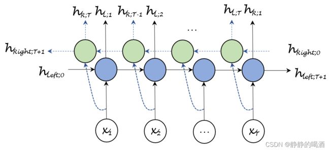
正常的$\text{GRU}$结构仅捕捉到了正向个时刻的序列信息；而双向结构是在正向的基础上，增加了反向的序列信息：
其中${\mathcal{H}}_{Single}$表示单向的序列信息;对应地，${\mathcal{H}}_{Bi}$表示双向的序列信息。
$$\begin{gathered} {\mathcal{H}}_{Single}=\{h_{\mathcal{L};1},h_{\mathcal{L};2},\cdots ,h_{\mathcal{L};\mathcal{T}}\} \\ {\mathcal{H}}_{Bi}=\{h_{\mathcal{L}\mathcal{R};1},h_{\mathcal{L}\mathcal{R};2},\cdots ,h_{\mathcal{L}\mathcal{R};\mathcal{T}}\} \end{gathered}$$
其中$h_{\mathcal{L}\mathcal{R};i}$表示第$i$时刻正、反方向序列信息的拼接$(\text{Concatenate})$结果，以此类推。
$$h_{\mathcal{L}\mathcal{R};i}=\left[h_{\mathcal{L}:i};h_{\mathcal{R};(\mathcal{T}+1-i)}\right]i=1,2\cdots ,\mathcal{T}$$
在代码中序列信息的描述表示如下：

import torch
from torch import nn as nn

BatchSize = 100
SeqLength = 10
EmbedSize = 8
NumHiddens = 16
NumLayers = 1

x = torch.randn(BatchSize,SeqLength,EmbedSize).permute(1,0,2)
SingleRNN = nn.GRU(EmbedSize,NumHiddens,NumLayers)
BiRNN = nn.GRU(EmbedSize,NumHiddens,NumLayers,bidirectional=True)
Output,State = SingleRNN(x)
print(x.shape)
print(Output.shape,State.shape)
BiOutput,BiState = BiRNN(x)
print(BiOutput.shape,BiState.shape)

序列信息的张量格式$(\text{Shape})$结果表示如下：

# Embedding Shape
torch.Size([10, 100, 8])
# SingleGRU.Output shape;FinalState shape
torch.Size([10, 100, 16]) torch.Size([1, 100, 16])
# BiGRU.Output shape;FinalState shape
torch.Size([10, 100, 32]) torch.Size([2, 100, 16])

可以观察一下，随意选取一个时刻。例如$\mathcal{T}=2$时刻。它对应的序列信息可表示为：
$$h_{\mathcal{L}\mathcal{R};2}=\left[h_{\mathcal{L};2};h_{\mathcal{R};\mathcal{T}-1}\right]$$
观察：

• $h_{\mathcal{L};2}$包含了正向序列数据$x^{(1)},x^{(2)}$的序列信息；
• $h_{\mathcal{R};\mathcal{T}-1}$包含了反向序列数据$x^{(\mathcal{T})},x^{(\mathcal{T}-1)},\cdots ,x^{(3)},x^{(2)}$的序列信息。这两组信息所组成的融合信息以$t=2$时刻为核心，将完整序列的序列信息都涵盖到了。

因而：$h_{\mathcal{L}\mathcal{R};2}$相比单向结构的$h_{\mathcal{L};2}$包含更加丰富的序列信息。

解码过程这里同样以第$2$时刻的解码为例：
这里'查询向量'使用$h_{\mathcal{D}}^{(1)},h_{\mathcal{D}}^{(2)}$都是有道理的。详见上一节——注意力机制的动机
$$y^{(2)}=\mathcal{G}(y^{(1)},{\mathcal{C}}_2,h_{\mathcal{D}}^{(2)})$$
描述生成$y^{(2)}$信息的复杂函数$\mathcal{G}(\cdot )$中，一共包含$3$类信息：

• 上一时刻的输出$y^{(1)}$；
• 当前时刻产生的序列信息$h_{\mathcal{D}}^{(2)}$;
• 通过注意力机制$(\text{Attention})$产生的，基于当前时刻具有注意力偏向的序列信息${\mathcal{C}}_2$。在双向结构中${\mathcal{C}}_2$表示如下：
  类似于上面单向网络，$(\text{Bi})s_{2j}$描述’解码器‘第$2$时刻的序列信息$h_{\mathcal{D}}^{(2)}$与‘编码器’第$j$时刻的双向序列信息${\mathcal{H}}_{Bi}^{(j)}=\left[h_{\mathcal{L};j};h_{\mathcal{R};(\mathcal{T}+1-j)}\right]$之间的评分结果。
  $$\{\begin{array}{l}\begin{array}{rl}(\text{Bi})s_{2j}& =\text{Score}({\mathcal{H}}_{Bi}^{(j)},h_{\mathcal{D}}^{(2)})\\ (\text{Bi}){\mathcal{S}}_2& =(\text{Bi})(s_{21},s_{22},\cdots ,s_{2\mathcal{T}}{)}^T\Leftarrow j=1,2,\cdots ,\mathcal{T}\\ {\mathcal{C}}_2& =[(\text{Bi}){\mathcal{S}}_2{]}^T\cdot {\mathcal{H}}_{Bi}\\ & =\sum _{j=1}^{\mathcal{T}}(\text{Bi})s_{2j}\cdot \left[h_{\mathcal{L};j};h_{\mathcal{R};(\mathcal{T}+1-j)}\right]\end{array}\end{array}$$

这种将${\mathcal{H}}_{Bi}$中的所有时刻的序列信息均做加权求和求解${\mathcal{C}}_2$的方式称作软注意力机制$(\text{Soft-Attention})$；

相反，与软注意力机制对应的是硬注意力机制$(\text{Hard-Attention})$。这种注意力机制将$\text{Score}$评分结果仅仅集中在若干个离散的序列信息中。也就是说，仅有$1$个/若干个结果有$\text{Score}$值，其余值均无影响。
但硬注意力机制比较困难，因为它在函数空间中并不处处可导。相反，软注意力机制在函数空间中处处可导，从而可以在反向传播过程中梯度进行传播。

注意力模型的数学推导整理

这里有一点啰嗦，不是一天写的，担待一下~

回顾机器翻译任务，最终目标是求解：给定输入序列数据$\mathcal{X}$以及解码器前$t-1$个时刻的输出信息$\{y^{(1)},y^{(2)},\cdots ,y^{(t-1)}\}$条件下，求解$t$时刻输出信息$y^{(t)}$的条件概率：
$$\mathcal{P}(y^{(t)}\mid \mathcal{X},y^{(1)},y^{(2)},\cdots ,y^{(t-1)})$$
从注意力机制的角度，将这个概率描述成函数的形式：
$$\mathcal{P}(y^{(t)}\mid \mathcal{X},y^{(1)},y^{(2)},\cdots ,y^{(t-1)})=\mathcal{G}(y^{(t-1)},h_{\mathcal{D}}^{(t)},{\mathcal{C}}_t)$$
其中$y^{(t-1)}$表示解码器$t-1$时刻的输出信息，作为$t$时刻输入的一部分；$h_{\mathcal{D}}^{(t)}$作为解码器当前时刻的序列信息，它表示为如下形式：
这里的‘复杂函数’$f(\cdot )$就是指循环神经网络系列的模型：$\text{LSTM,GRU,RNN}$
$$h_{\mathcal{D}}^{(t)}=f(y^{(t-1)},h_{\mathcal{D}}^{(t-1)},{\mathcal{C}}_t)$$
关于${\mathcal{C}}_t$就是编码器各时刻的输出与相应$\text{Score}$的加权求和结果：
这里仍然用‘双向循环网络’结构示例。
$${\mathcal{C}}_t=\sum _{j=1}^{\mathcal{T}}{s}_{tj}\cdot \left[h_{\mathcal{L};j};h_{\mathcal{R};(\mathcal{T}+1-j)}\right]$$
关于编码器第$j$个时刻的输出$\left[h_{\mathcal{L};j};h_{\mathcal{R};(\mathcal{T}+1-j)}\right]$与解码器$t$时刻的序列信息$h_{\mathcal{D}}^{(t)}$之间$\text{Score}$结果$s_{tj}$的计算共分两个步骤：

• 用内积、或者构建神经网络的方式求解$\text{Score}$结果；
  关于两种方法的描述详见上一节：注意力机制的动机
  $$e_{tj}=\text{Score}(h_{\mathcal{D}}^{(t)};\left[h_{\mathcal{L};j};h_{\mathcal{R};(\mathcal{T}+1-j)}\right])j=1,2,\cdots ,\mathcal{T}$$
  这里以构建神经网络为例，描述$\text{Score}$输出${\mathcal{E}}_t(e_{t1},e_{t2},\cdots ,e_{t\mathcal{T}}{)}^T$的执行过程：

  • 将$h_{\mathcal{D}}^{(t)}$(或者$h_{\mathcal{D}}^{(t-1)}$)与编码器输出$\left[h_{\mathcal{L};j};h_{\mathcal{R};(\mathcal{T}+1-j)}\right]$之间做向量拼接$(\text{Concatenate})$，并作为$\text{Attn}$线性计算层的输入：
    $$\begin{array}{rl}{\mathcal{O}}_t& =\text{Attn}\left(h_{\mathcal{D}}^{(t)},\left[h_{\mathcal{L};j};h_{\mathcal{R};(\mathcal{T}+1-j)}\right]\right)\\ & ={\mathcal{W}}_{\text{Attn}}\cdot \left[\text{Concat}\left(h_{\mathcal{D}}^{(t)},\left[h_{\mathcal{L};j};h_{\mathcal{R};(\mathcal{T}+1-j)}\right]\right)\right]+b_{\text{Attn}}\end{array}$$
  • $\text{Attn}$层的激活函数选择$\text{Tanh}$激活函数：
    个人理解：在数值稳定性、模型初始化与激活函数中介绍了激活函数的本质。激活函数的目的是：维持低次项数值稳定的基础上(激活函数的线性近似区逼近$y=x$,即恒等映射),去学习高次项特征。
    关于激活函数作用的输出分布${\mathcal{O}}^{(t)}$,从物理意义的角度，它仅仅是$h_{\mathcal{D}}^{(t)}$与$\left[h_{\mathcal{L};j};h_{\mathcal{R};(\mathcal{T}+1-j)}\right]$之间关系的一个‘抽象’描述。但不可否认的是：${\mathcal{O}}^{(t)}$中的分量对表示两者之间关系存在实际价值。如果使用$\text{ReLU}$激活函数去稀疏这个信息(使一部分分量置$0$)，个人认为不太可取。
    $${\mathcal{O}}_t=\text{Tanh}({\mathcal{O}}_t)$$
    其次，从泰勒公式的角度，明显能够看出$\text{Tanh}$激活函数在低次项数值的映射结果中，它比$\text{Sigmoid}$函数更接近‘恒等映射’:
    $$\{\begin{array}{l}\begin{array}{rl}\text{Sigmoid}(x)& =\frac{1}{2}+\frac{1}{4}x-\frac{1}{48}{x}^3+\mathcal{O}(x^5)\\ \text{Tanh}(x)& =0+x-\frac{1}{3}{x}^3+\mathcal{O}(x^5)\end{array}\end{array}$$
    并且$\text{Tanh}$激活函数的映射范围是$(-1,1)$,因此关于一些信息的非线性映射，$\text{Tanh}$激活函数效果更优。
  • $\text{Tanh}$函数映射结束后，${\mathcal{O}}_t$中每一个分量的输出大小是解码器的隐藏层神经元数量。在此基础上，使用神经元权重$\mathcal{V}$学习${\mathcal{O}}_t$的特征信息，并将${\mathcal{O}}_t$中每一个分量映射为标量信息：
    $${\mathcal{E}}_t={\mathcal{V}}^T{\mathcal{O}}_t\mathcal{V}\in {\mathbb{R}}^{{\mathcal{N}}_{De}\times 1}$$

• 计算出的关于$\text{Score}$的结果向量${\mathcal{E}}_t=(e_{t1},e_{t2},\cdots ,e_{t\mathcal{T}}{)}^T$不能直接使用，需要将其映射成概率形式——$\text{Softmax}$函数：
  $$\{\begin{array}{l}\begin{array}{rl}{s}_{tj}& =\frac{\exp (e_{tj})}{\begin{array}{r}\sum _{k=1}^{\mathcal{T}}\exp (e_{tk})\end{array}}j=1,2,\cdots ,\mathcal{T}\\ {\mathcal{S}}_t& =(s_{t1},s_{t2},\cdots ,s_{t\mathcal{T}}{)}^T\end{array}\end{array}$$
  最终通过线性计算，求出${\mathcal{C}}_t$。

至此，关于$3$个信息：$y^{(t-1)},h_{\mathcal{D}}^{(t)},{\mathcal{C}}_t$都已求出，针对$3$个信息构建神经网络，对$y^{(t)}$的后验概率$\mathcal{G}(y^{(t-1)},h_{\mathcal{D}}^{(t)},{\mathcal{C}}_t)$进行预测：

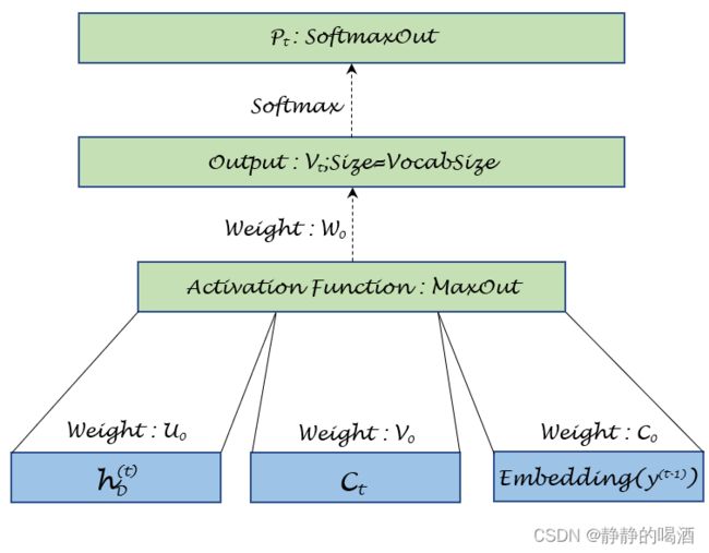
对应函数的执行过程表示如下：

• 需要注意的是：这里的$y^{(t-1)}$是上一时刻的输出特征，在作为下一时刻输入时，需将其重新转化为$\text{Embedding}$向量信息。
• 关于$\text{MaxOut}$激活函数，该函数一次比对若干个连续结果的大小，并取出其中最大的元素进行输出;移动窗口，执行下一次比较。其效果类似于卷积神经网络中的最大池化层,用于“保留信息的基础上，降低特征维数。”这里使用窗口大小为$2$进行示例。

$$\{\begin{array}{l}\begin{array}{rl}{h}_t& ={\mathcal{U}}_o\cdot h_{\mathcal{D}}^{(t)}+{\mathcal{V}}_o\cdot {\mathcal{C}}_t+{\mathcal{C}}_o\cdot \text{Embedding}(y^{(t-1)})\\ h_t& =\max \{h_{t;2i-1},h_{t;2i}\}\\ {\mathcal{V}}_t& ={\mathcal{W}}_o\cdot h_t\\ {\mathcal{P}}_t& =\text{Softmax}({\mathcal{V}}_t)\end{array}\end{array}$$
最终使用$\text{Argmax}$选择出对应位置的词语结果即可。

相关参考：
seq2seq与attention机制
激活函数($\text{ReLU,Swish,Maxout}$)
Seq2seq进阶，双向GRU