【R语言实例】物种分布模型介绍

作者简介： 本文作者系大学统计学专业教师，多年从事统计学的教学科研工作，在随机过程、统计推 断、机器学习领域有深厚的理论积累与应用实践。个人主页

1. 背景知识

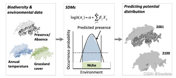
物种分布模型(species distribution models, SDM)是数量生态学里的一个流行的分析工具。SDM普遍使用数理模型评估全球生态变化对于物种迁移的潜在影响。它的优势体现在：有很多容易使用的软件工具与参考指南，对数据的要求较低。

1.1 SDM 输入

SDM要求输入有地理坐标参考的生物多样性观测。比如，个体坐标、物种的presence, 物种数量、物种的richness, 响应变量等。此外，地理图层、环境信息也可以作为SDM的输入。这些信息通常以数码格式保存。

1.2 在线数据库

• GBIF the Global Biodiversity Information Facility
• OBIS Ocean Biodiversity Information System
• Movebank animal tracking data
• WorldClim global climate data

利用这些数据，我们可以建立统计机器学习模型，描述特定地点的生物多样性观测与气候条件的关系，然后把模型投射到可利用的环境图层上，在时空上做预测。

2. SDM 实例

2.1 一个例子：Ring Ouzel

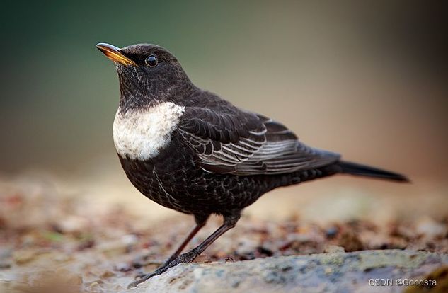
环颈鸫(Ring Ouzel), 鸫属的一种鸟类，生活在欧洲，与乌鸫有亲缘关系。其成年雄性通体黑色，胸部有白色月牙标记，有黄色的喙。雌性与其相似，但颜色较淡，胸部无白色月牙。

在这个实例里，我们想评估气候变化对栖息在瑞士的环颈鸫种群的影响。环颈鸫主要栖息地在瑞士北方的阿尔卑斯山脉，对气候变暖比较敏感，另外还有其它的影响指标。上世纪90年代以来，环颈鸫的种群密度已经下降，而在海拔2000米以上的群体仍然维持稳定。在邻近国家，种群假定是稳定的。
瑞士鸟类协会收集了两类环颈鸫分布数据。这里，我们研究气候对环颈鸫分布的影响。为此，选取了5个最重要的预测变量。

• bio5 = maximum temperature of the warmest month,
• bio2 = mean diurnal range,
• bio14 = precipitation of driest month,
• std = standard deviation of vegetation height,
• rad = annual total radiation.

为了理解不同的统计模型/算法的区别，我们拟合简单的广义线性模型与随机森林。模型输出的是当前与未来分布概率图，潜在的分布二值图谱。

2.2 数据准备

在这一步，收集处理真实的环颈鸫生物多样性与环境数据。对于生物多样性数据，物种的presence信息可以直接观测到，而absence信息作为presence数据的对比数据很难获得。这种情况下，我们需要充分的background数据，或者pseudo-absence数据。准备好后，首先导入数据。

avi_dat <- read.table('data/Data_SwissBreedingBirds.csv', header=T, sep=',')

summary(avi_dat)

该数据框由56个鸟类物种的2,535条presence-absence信息记录、52个环境预测变量组成。其中，数据的70%用作单一物种分布建模，其余30%用作检验预测。下面，我们缩减数据框到相关的变量列。

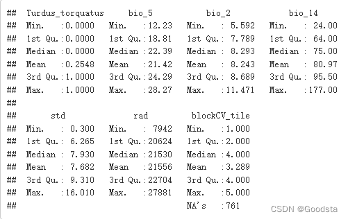
avi_cols <- c('Turdus_torquatus', 'bio_5', 'bio_2', 'bio_14', 'std', 'rad', 'blockCV_tile')

avi_df <- data.frame(avi_dat)[avi_cols]

summary(avi_df)

为了定位对应当前气候的物种分布，以及未来气候下的潜在分布图，我们使用WorldClim数获得生物气候变量值。该数据可以直接从R环境下载。

library(raster)

# Please note that you have to set download=T if you haven't downloaded the data before:
bio_curr <- getData('worldclim', var='bio', res=0.5, lon=5.5, lat=45.5, path='data')[[c(2,5,14)]]

# Please note that you have to set download=T if you haven't downloaded the data before:
bio_fut <- getData('CMIP5', var='bio', res=0.5, lon=5.5, lat=45.5, rcp=45, model='NO', year=50, path='data', download=F)[[c(2,5,14)]]

我们使用背景mask定位瑞士坐标，这需要重新投射worldclim层。

# A spatial mask of Switzerland in Swiss coordinates
bg <- raster('/vsicurl/https://damariszurell.github.io/SDM-Intro/CH_mask.tif')

# The spatial extent of Switzerland in Lon/Lat coordinates is roughly:
ch_ext <- c(5, 11, 45, 48)

# Crop the climate layers to the extent of Switzerland
bio_curr <- crop(bio_curr, ch_ext)

# Re-project to Swiss coordinate system and clip to Swiss political bounday
bio_curr <- projectRaster(bio_curr, bg)
bio_curr <- resample(bio_curr, bg)
bio_curr <- mask(bio_curr, bg)
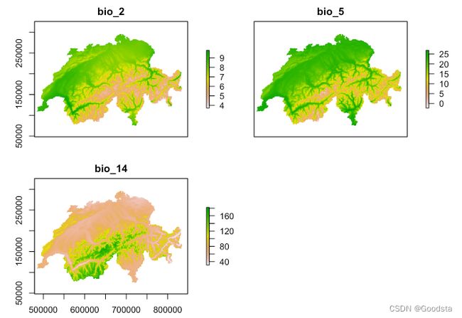
names(bio_curr) <- c('bio_2', 'bio_5', 'bio_14')

# For storage reasons the temperature values in worldclim are multiplied by 10. For easier interpretability, we change it back to °C.
bio_curr[[1]] <- bio_curr[[1]]/10
bio_curr[[2]] <- bio_curr[[2]]/10

# Repeat above steps for future climate layers
bio_fut <- crop(bio_fut, ch_ext)
bio_fut <- projectRaster(bio_fut, bg)
bio_fut <- resample(bio_fut, bg)
bio_fut <- mask(bio_fut, bg)
names(bio_fut) <- c('bio_2', 'bio_5', 'bio_14')
bio_fut[[1]] <- bio_fut[[1]]/10
bio_fut[[2]] <- bio_fut[[2]]/10

plot(bio_curr)

2.3 模型拟合

我们拟合一个参数回归方法广义线性模型(GLM)，一个机器学习方法随机森林(RF)。然后，探索GLM的模型系数，RF的变量重要性，画出响应曲线。计算得到气候变量的相关系数|r|<0.7, 故不必考虑变量间的多重共线性问题。

2.3.1 广义线性模型

# Fit GLM
m_glm <- glm( Turdus_torquatus ~ bio_2 + I(bio_2^2) + bio_5 + I(bio_5^2) + bio_14 + I(bio_14^2), family='binomial', data=avi_df)

summary(m_glm)

# Install the mecofun package
library(devtools)
devtools::install_git("https://gitup.uni-potsdam.de/macroecology/mecofun.git")
# Load the mecofun package
library(mecofun)

# Names of our variables:
pred <- c('bio_2', 'bio_5', 'bio_14')

# We want three panels next to each other:
par(mfrow=c(1,3)) 

# Plot the partial responses
partial_response(m_glm, predictors = avi_df[,pred])

library(RColorBrewer)
library(lattice)

# We prepare the response surface by making a dummy data set where two predictor variables range from their minimum to maximum value, and the remaining predictor is kept constant at its mean:
xyz <- data.frame(expand.grid(seq(min(avi_df[,pred[1]]),max(avi_df[,pred[1]]),length=50), seq(min(avi_df[,pred[2]]),max(avi_df[,pred[2]]),length=50)), mean(avi_df[,pred[3]]))
names(xyz) <- pred

# Make predictions
xyz$z <- predict(m_glm, xyz, type='response')
summary(xyz)

# Make a colour scale
cls <- colorRampPalette(rev(brewer.pal(11, 'RdYlBu')))(100)

# plot 3D-surface
wireframe(z ~ bio_2 + bio_5, data = xyz, zlab = list("Occurrence prob.", rot=90),
    drape = TRUE, col.regions = cls, scales = list(arrows = FALSE), zlim = c(0, 1), 
    main='GLM', xlab='bio_2', ylab='bio_5', screen=list(z = 120, x = -70, y = 3))

# Plot inflated response curves:
par(mfrow=c(1,3)) 
inflated_response(m_glm, predictors = avi_df[,pred], method = "stat6", lwd = 3, main='GLM') 

2.3.2 随机森林

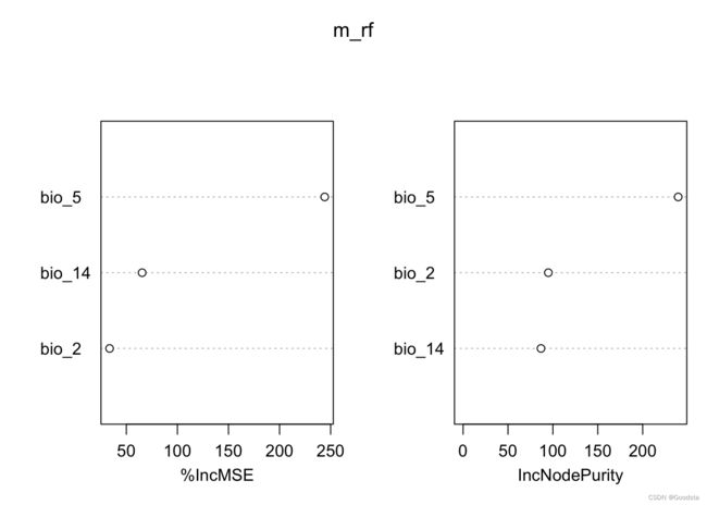
随机森林是一类bagging(bootstrap aggregation)算法，它平均多个不同的分类回归树CARTs输出。这样，RF本质上是交叉验证法。RF的另一个重要作用是评价预测变量的重要性，即，预测变量对模型的相对贡献。

library(randomForest)

# Fit RF
(m_rf <- randomForest( x=avi_df[,2:4], y=avi_df[,1], ntree=1000, nodesize=10, importance =T))

# Variable importance:
importance(m_rf,type=1)
varImpPlot(m_rf)

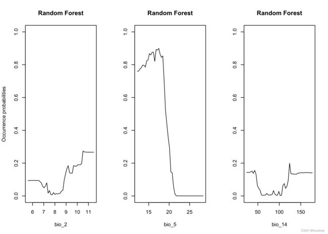
# Now, we plot response curves in the same way as we did for GLMs above:
par(mfrow=c(1,3)) 
partial_response(m_rf, predictors = avi_df[,pred], main='Random Forest')

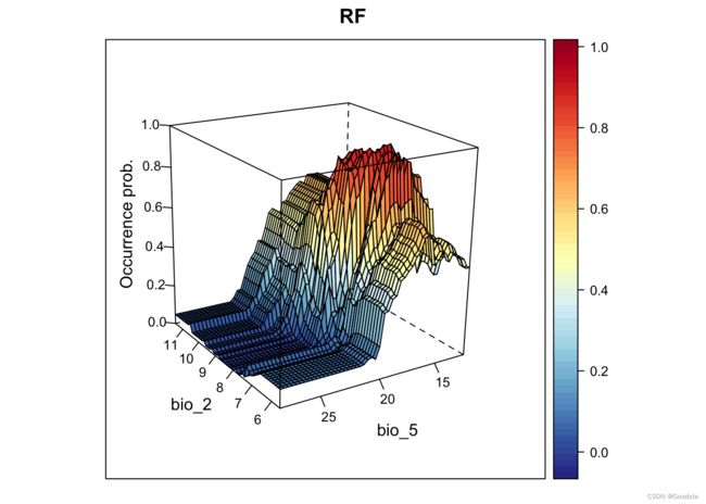
# Plot the response surface:
xyz$z <- predict(m_rf, xyz)   # Note that we created the xyz data.frame in the GLM example above
wireframe(z ~ bio_2 + bio_5, data = xyz, zlab = list("Occurrence prob.", rot=90),
    drape = TRUE, col.regions = cls, scales = list(arrows = FALSE), zlim = c(0, 1), 
    main='RF', xlab='bio_2', ylab='bio_5', screen=list(z = 120, x = -70, y = 3))

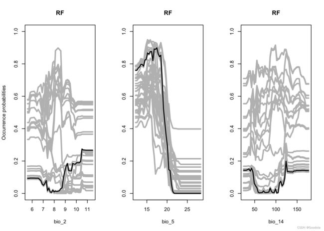
# Plot inflated response curves:
par(mfrow=c(1,3)) 
inflated_response(m_rf, predictors = avi_df[,pred], method = "stat6", lwd = 3, main='RF') 

2.4 模型评价

我们使用交叉验证法评价模型的预测表型。用到的评价测度有：

• AUC: the area underROC
• TSS: the true skill statistic, the sum of sensitivity and specificity
• sensitivity: the true positive rate
• specificity: the true negative rate

另外，为了做二值预测，还需要估计最优的阈值。我们使用最大化 TSS的阈值。

# Make cross-validated predictions for GLM:
crosspred_glm <- mecofun::crossvalSDM(m_glm, traindat= avi_df[!is.na(avi_df$blockCV_tile),], colname_pred=pred, colname_species = "Turdus_torquatus", kfold= avi_df[!is.na(avi_df$blockCV_tile),'blockCV_tile'])

# Make cross-validated predictions for RF:
crosspred_rf <- mecofun::crossvalSDM(m_rf, traindat= avi_df[!is.na(avi_df$blockCV_tile),], colname_pred=pred, colname_species = "Turdus_torquatus", kfold= avi_df[!is.na(avi_df$blockCV_tile),'blockCV_tile'])

# Look at correlation between GLM and RF predictions:
plot(crosspred_glm, crosspred_rf, pch=19, col='grey35')

eval_glm <- mecofun::evalSDM(observation = avi_df[!is.na(avi_df$blockCV_tile),1], predictions = crosspred_glm)

eval_rf <- mecofun::evalSDM(observation = avi_df[!is.na(avi_df$blockCV_tile),1], predictions = crosspred_rf)

集成GLM, RF组合模型，取中位数。

# Derive median predictions:
crosspred_ens <- apply(data.frame(crosspred_glm, crosspred_rf),1,median)

# Evaluate ensemble predictions
eval_ens <- mecofun::evalSDM(observation = avi_df[!is.na(avi_df$blockCV_tile),1], predictions = crosspred_ens)

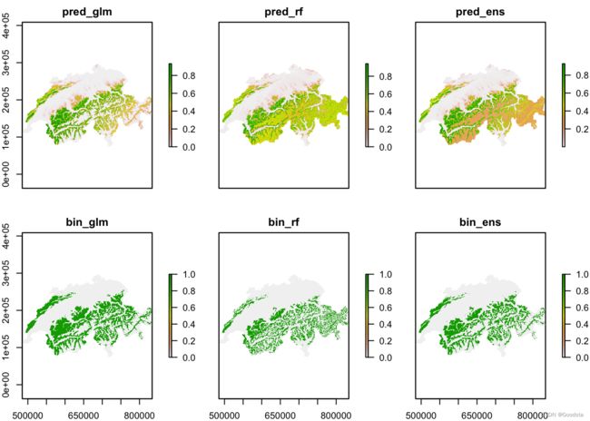
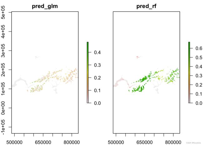
2.5 预测

我们的目的是定位环颈鸫当前的分布，当气候改变时，与未来分布比较。简单起见，我们只选择一种气候模型和一个代表性的RCP(representative concentration pathway)

# Make predictions to current climate:
bio_curr_df <- data.frame(rasterToPoints(bio_curr))
bio_curr_df$pred_glm <- mecofun::predictSDM(m_glm, bio_curr_df)
bio_curr_df$pred_rf <- mecofun::predictSDM(m_rf, bio_curr_df)
bio_curr_df$pred_ens <- apply(bio_curr_df[,-c(1:5)],1,median)

# Make binary predictions:
bio_curr_df$bin_glm <- ifelse(bio_curr_df$pred_glm > eval_glm$thresh, 1, 0)
bio_curr_df$bin_rf <- ifelse(bio_curr_df$pred_rf > eval_rf$thresh, 1, 0)
bio_curr_df$bin_ens <- ifelse(bio_curr_df$pred_ens > eval_ens$thresh, 1, 0)

# Make raster stack of predictions:
r_pred_curr <- rasterFromXYZ(bio_curr_df[,-c(3:5)])
plot(r_pred_curr)

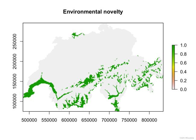
对于未来的气候层，我们量化新环境。

# Assess novel environments in future climate layer:
bio_fut_df <- data.frame(rasterToPoints(bio_fut))
# Values of 1 in the eo.mask will indicate novel environmental conditions
bio_fut_df$eo_mask <- mecofun::eo_mask(avi_df[,pred], bio_fut_df[,pred])
plot(rasterFromXYZ(bio_fut_df[,-c(3:5)]), main='Environmental novelty')

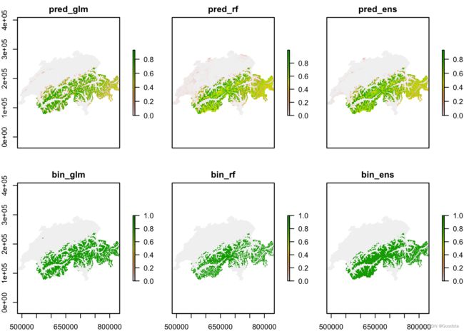
# Make predictions to future climate:
bio_fut_df$pred_glm <- mecofun::predictSDM(m_glm, bio_fut_df)
bio_fut_df$pred_rf <- mecofun::predictSDM(m_rf, bio_fut_df)
bio_fut_df$pred_ens <- apply(bio_fut_df[,-c(1:5)],1,median)

# Make binary predictions:
bio_fut_df$bin_glm <- ifelse(bio_fut_df$pred_glm > eval_glm$thresh, 1, 0)
bio_fut_df$bin_rf <- ifelse(bio_fut_df$pred_rf > eval_rf$thresh, 1, 0)
bio_fut_df$bin_ens <- ifelse(bio_fut_df$pred_ens > eval_ens$thresh, 1, 0)

# Make raster stack of predictions:
r_pred_fut <- rasterFromXYZ(bio_fut_df[,-c(3:5)])
plot(r_pred_fut[[-1]])

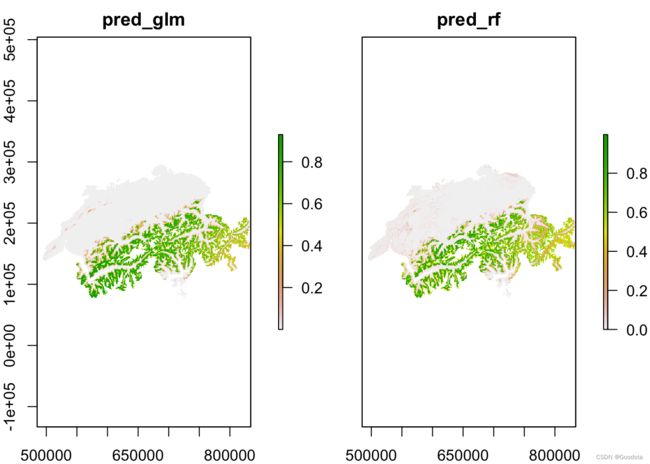
# Predictions to analogous climates:
bio_analog_df <- bio_fut_df[,c('x','y','pred_glm','pred_rf')]
bio_analog_df[bio_fut_df$eo_mask>0,c('pred_glm','pred_rf')] <- NA
plot(rasterFromXYZ(bio_analog_df))

# Predictions to novel climates:
bio_novel_df <- bio_fut_df[,c('x','y','pred_glm','pred_rf')]
bio_novel_df[bio_fut_df$eo_mask==0,c('pred_glm','pred_rf')] <- NA
plot(rasterFromXYZ(bio_novel_df))

完