cs231n assignment3解析
cs231n-assignment3解析
前言:每年的作业都差不多,但是有些地方有微小改动,比如将循环的内容单独作为一个函数,核心内容其实都是一样的。
作业要求见该网站:https://cs231n.github.io/assignments2017/assignment3/
cs231n的三次作业都放在了我的GitHub仓库,可以进去查看。
由于我是看完课程再写的作业,所以我一般把一个文件里要写的函数部分全部写完,该博文也是这么书写的,没有按照Q1、Q2……题中所需的顺序一个个写函数,见谅见谅。
数据准备
这一部分使用的是 Microsoft COCO dataset ,可以直接进入下面的网址:http://cs231n.stanford.edu/coco_captioning.zip 下载数据,解压后放入工作区直接使用即可。
rnn_layers.py
rnn_step_forward()
由于 RNN 的前向传播公式是:
h t + 1 = t a n h ( W x x t + 1 + W h h t + b ) h_{t+1} = tanh(W_xx_{t+1} + W_hh_t + b) ht+1=tanh(Wxxt+1+Whht+b)因此直接使用矩阵乘法计算即可。
def rnn_step_forward(x, prev_h, Wx, Wh, b):
    """
    Run the forward pass for a single timestep of a vanilla RNN that uses a tanh
    activation function.

    The input data has dimension D, the hidden state has dimension H, and we use
    a minibatch size of N.

    Inputs:
    - x: Input data for this timestep, of shape (N, D).
    - prev_h: Hidden state from previous timestep, of shape (N, H)
    - Wx: Weight matrix for input-to-hidden connections, of shape (D, H)
    - Wh: Weight matrix for hidden-to-hidden connections, of shape (H, H)
    - b: Biases of shape (H,)

    Returns a tuple of:
    - next_h: Next hidden state, of shape (N, H)
    - cache: Tuple of values needed for the backward pass.
    """
    next_h, cache = None, None
    ##############################################################################
    # TODO: Implement a single forward step for the vanilla RNN. Store the next  #
    # hidden state and any values you need for the backward pass in the next_h   #
    # and cache variables respectively.                                          #
    ##############################################################################
    next_h = np.tanh(np.dot(x, Wx) + np.dot(prev_h, Wh) + b)
    cache = (next_h, Wx, Wh, x, prev_h, b)
    ##############################################################################
    #                               END OF YOUR CODE                             #
    ##############################################################################
    return next_h, cache
rnn_step_backward()
这里一共要计算出 dx,dpre_h,dWx,dWh,db
tanh激活函数
tanh激活函数的定义是: t a n h ( x ) = e x − e − x e x + e − x tanh(x) = \frac{e^x - e^{-x}}{e^x + e^{-x}} tanh(x)=ex+e−xex−e−x其对于自变量 x 的导数为: t a n h ′ ( x ) = 1 − t a n h 2 ( x ) tanh^{'}(x) = 1-tanh^2(x) tanh′(x)=1−tanh2(x)(可以求导一下,结果和这个公式是一样的,但是这么书写和计算更为简洁)
求导计算
注意这是一个含有 tanh 激活函数的复合函数,因此以求 dx 为例,应: d x = d n e x t _ h ∗ d t a n h ∗ ∂ t a n h ∂ x dx = dnext\_h * dtanh * \frac{\partial{tanh}}{\partial{x}} dx=dnext_h∗dtanh∗∂x∂tanh所以程序应写为:
def rnn_step_backward(dnext_h, cache):
    """
    Backward pass for a single timestep of a vanilla RNN.

    Inputs:
    - dnext_h: Gradient of loss with respect to next hidden state
    - cache: Cache object from the forward pass

    Returns a tuple of:
    - dx: Gradients of input data, of shape (N, D)
    - dprev_h: Gradients of previous hidden state, of shape (N, H)
    - dWx: Gradients of input-to-hidden weights, of shape (D, H)
    - dWh: Gradients of hidden-to-hidden weights, of shape (H, H)
    - db: Gradients of bias vector, of shape (H,)
    """
    dx, dprev_h, dWx, dWh, db = None, None, None, None, None
    ##############################################################################
    # TODO: Implement the backward pass for a single step of a vanilla RNN.      #
    #                                                                            #
    # HINT: For the tanh function, you can compute the local derivative in terms #
    # of the output value from tanh.                                             #
    ##############################################################################
    next_h, Wx, Wh, x, prev_h, b = cache
    # temp_x = np.dot(x, Wx) + np.dot(prev_h, Wh) + b
    dtanh = dnext_h * (1 - next_h**2)
    dx = np.dot(dtanh, Wx.T)
    dprev_h = np.dot(dtanh, Wh.T)
    dWx = np.dot(x.T, dtanh)
    dWh = np.dot(prev_h.T, dtanh)
    db = np.sum(dtanh, 0)
    ##############################################################################
    #                               END OF YOUR CODE                             #
    ##############################################################################
    return dx, dprev_h, dWx, dWh, db
rnn_forward()
这个函数是 RNN 的总体前向传播的函数,输入 x 加入了时间维度,需要嵌套调用rnn_step_forward() 函数。其输出 h 是一个数组,记录了 RNN 网络每个时刻的状态。我们使用 for 循环模拟时间的推移,因此在数组 h 中存储的维度是 [T, N, H] ,这不是我们想要的维度顺序,因此使用 transpose() 函数来变换维度顺序。
其中 h 0 h_0 h0 RNN 网络的初始状态。
def rnn_forward(x, h0, Wx, Wh, b):
    """
    Run a vanilla RNN forward on an entire sequence of data. We assume an input
    sequence composed of T vectors, each of dimension D. The RNN uses a hidden
    size of H, and we work over a minibatch containing N sequences. After running
    the RNN forward, we return the hidden states for all timesteps.

    Inputs:
    - x: Input data for the entire timeseries, of shape (N, T, D).
    - h0: Initial hidden state, of shape (N, H)
    - Wx: Weight matrix for input-to-hidden connections, of shape (D, H)
    - Wh: Weight matrix for hidden-to-hidden connections, of shape (H, H)
    - b: Biases of shape (H,)

    Returns a tuple of:
    - h: Hidden states for the entire timeseries, of shape (N, T, H).
    - cache: Values needed in the backward pass
    """
    h, cache = None, None
    ##############################################################################
    # TODO: Implement forward pass for a vanilla RNN running on a sequence of    #
    # input data. You should use the rnn_step_forward function that you defined  #
    # above. You can use a for loop to help compute the forward pass.            #
    ##############################################################################
    T = x.shape[1]
    prev_h = h0
    h, cache = [], []
    for t in range(T):
        next_h, next_cache = rnn_step_forward(x[:, t, :], prev_h, Wx, Wh, b)
        h.append(next_h)
        cache.append(next_cache)
        prev_h = next_h
    #! 注意上面的h输出的维度是[T, N, H],因为最里面的循环是循环时间的,所以第一维是T
    h = np.array(h).transpose(1, 0, 2)
    ##############################################################################
    #                               END OF YOUR CODE                             #
    ##############################################################################
    return h, cache
rnn_backward()
这个函数是 RNN 的总体反向传播的函数,输入 x 加入了时间维度,需要嵌套调用rnn_step_backward() 函数。
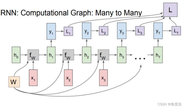
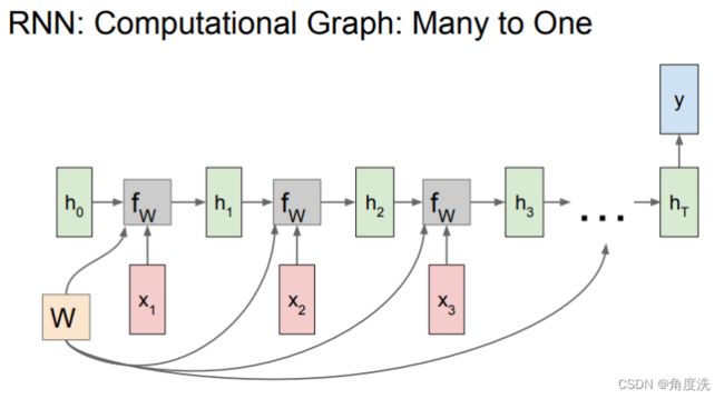
里面需要注意的是在调用 rnn_step_backward() 函数时传入的 dnext_h 参数。dnext_h 是需要叠加从上面(也就是h,即总体的状态的梯度)和右边(next_h)传来的梯度,而不是单纯只传入下一个状态(next_h)的梯度,结合下面 RNN 网络 many-to-many 和 many-to-one 和 one-to-one 的网络示意图,当前时刻的状态有参与到所有状态的梯度的计算中,体现在dh[:, t, :],也有传播到下一个状态next_h,再计算下一个状态的损失,所以要叠加h的和next_h的梯度
def rnn_backward(dh, cache):
    """
    Compute the backward pass for a vanilla RNN over an entire sequence of data.

    Inputs:
    - dh: Upstream gradients of all hidden states, of shape (N, T, H)

    Returns a tuple of:\

    - dx: Gradient of inputs, of shape (N, T, D)
    - dh0: Gradient of initial hidden state, of shape (N, H)
    - dWx: Gradient of input-to-hidden weights, of shape (D, H)
    - dWh: Gradient of hidden-to-hidden weights, of shape (H, H)
    - db: Gradient of biases, of shape (H,)
    """
    dx, dh0, dWx, dWh, db = None, None, None, None, None
    ##############################################################################
    # TODO: Implement the backward pass for a vanilla RNN running an entire      #
    # sequence of data. You should use the rnn_step_backward function that you   #
    # defined above. You can use a for loop to help compute the backward pass.   #
    ##############################################################################
    N, T, H = dh.shape
    D = cache[0][1].shape[0]
    ddh = np.zeros((N, H))
    dx, dWx, dWh, db = [], np.zeros((D, H)), np.zeros((H, H)), np.zeros(H)

    for t in range(T - 1, -1, -1):
        ddx, ddh, ddWx, ddWh, ddb = rnn_step_backward(dh[:, t, :] + ddh, cache[t]) #! 注意导数是叠加从上面和右边传来的梯度,结合笔记里的RNN的图,当前时刻的状态有参与到最终损失的计算中,体现在dh[:, t, :],也有传播到下一个状态next_h,再计算下一个状态的损失,所以要叠加h的和next_h的梯度
        dx.append(ddx)
        dWx = dWx + ddWx #! 由于在每一个时间 t 用的都是相同的系数 Wx 和 Wh ,所以梯度应当加和起来
        dWh = dWh + ddWh
        db = db + ddb
    dh0 = ddh
    dx = np.array(dx[::-1]).transpose(1, 0, 2) #! 注意这里由于时间是从后向前传递的,因此排在 dx 列表前面的是后面时间的梯度,排在后面的是前面的时间的梯度,因此要用[::-1]来调换一下方向,而使用 for 循环得到的 dx 维度是 [T, N, H] ,因此还要使用 transpose 来调换一下方向
    ##############################################################################
    #                               END OF YOUR CODE                             #
    ##############################################################################
    return dx, dh0, dWx, dWh, db
word_embedding_forward()
word_embedding的知识我参考总结了一下下面这篇博文:https://blog.csdn.net/weixin_42214778/article/details/105182423
word_embedding功能描述
在把我们的输入送给RNN之前,我们还需要做一个额外的操作,那就是word embedding,word embedding 简单来说就是将一个单词表示成一个向量的形式,因为我们神经网络要训练,需要我们把扔进去的单词先转换成常见的矩阵形式,再丢给神经网络。这里需要实现的是 word_embedding_forward 和 word_embedding_backward 两个函数。
参数解释
这里的输入有:1、x:其维度是(N,T),我理解为共有 N 个样本,每个样本有 T 个时间过程,其元素内容就是单词在词表中的下标;2、W:这是一个词表,其维度是(V,D),我理解为是一张每个单词相应的矩阵形式表,共有 V 个单词,每个单词对应 D 个特征。
这里的输出就是输入单词的矩阵形式:维度是(N,T,D),N 个样本,T 个时间阶段,每个单词 D 个特征。
由于输入 x 的元素内容就是单词在词表中的下标,因此可以直接使用 W[x, : ] 来取出相应单词的矩阵表示。
def word_embedding_forward(x, W):
    """
    Forward pass for word embeddings. We operate on minibatches of size N where
    each sequence has length T. We assume a vocabulary of V words, assigning each
    to a vector of dimension D.

    Inputs:
    - x: Integer array of shape (N, T) giving indices of words. Each element idx
      of x muxt be in the range 0 <= idx < V.
    - W: Weight matrix of shape (V, D) giving word vectors for all words.

    Returns a tuple of:
    - out: Array of shape (N, T, D) giving word vectors for all input words.
    - cache: Values needed for the backward pass
    """
    out, cache = None, None
    ##############################################################################
    # TODO: Implement the forward pass for word embeddings.                      #
    #                                                                            #
    # HINT: This can be done in one line using NumPy's array indexing.           #
    ##############################################################################
    #* 个人理解是输入的 x 有 N 个样本,每个样本 T 个时间过程,其元素内容就是单词,W 是长度为 V 的词表,每个词对应 D 个特征
    out = W[x, :] #! 输出的就是词表中在 x 的元素表示的下标上的长度为 D 的特征————shape (N, T, D)
    cache = (W, x)
    ##############################################################################
    #                               END OF YOUR CODE                             #
    ##############################################################################
    return out, cache
word_embedding_backward()
由于 word_embedding 在前向传播的时候输出是 out = W[x, :] ,因此变量 out 在对 W 求导时只需要在 dW 矩阵上以 x 矩阵元素值为下标加上 dout 的值,因为 out 只依赖于 W 在特定位置(即 x 的元素所表示的下标)的值, out 对 W 求导之后系数是 1 ,所以只要在特定位置加上 dout 的值就行。
需要注意的时使用了一个函数 np.add.at(A, B, C),其使用方式是在 A 中 B 下标的位置上加上 C 的值,注意 C 可能是一个矩阵,加上一个矩阵的值也不足为奇,因为 B 表示的下标位置也不一定是最后一维。
def word_embedding_backward(dout, cache):
    """
    Backward pass for word embeddings. We cannot back-propagate into the words
    since they are integers, so we only return gradient for the word embedding
    matrix.

    HINT: Look up the function np.add.at

    Inputs:
    - dout: Upstream gradients of shape (N, T, D)
    - cache: Values from the forward pass

    Returns:
    - dW: Gradient of word embedding matrix, of shape (V, D).
    """
    dW = None
    ##############################################################################
    # TODO: Implement the backward pass for word embeddings.                     #
    #                                                                            #
    # Note that Words can appear more than once in a sequence.                   #
    # HINT: Look up the function np.add.at                                       #
    ##############################################################################
    W, x = cache
    dW = np.zeros_like(W)
    np.add.at(dW, x, dout) #! 在 dW 矩阵上根据 x 矩阵作为下标加上 dout 的值,因为 out 只依赖于 W 在特定位置(即 x 的元素所表示的 W 的下标)的值, out 对 W 求导之后系数是 1 ,所以只要在特定位置加上 dout 的值就行
    ##############################################################################
    #                               END OF YOUR CODE                             #
    ##############################################################################
    return dW
lstm_step_forward()
LSTM前向传播公式及流程示意图
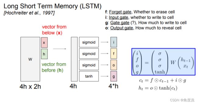
⊙表示矩阵对应位置元素相乘,c 是 cell state,h 是每个时间阶段的状态,注意区分 c 和 h
这里图上 W W W 能直接矩阵乘 ( h t − 1 x t ) \begin{pmatrix}h_{t - 1}\\x_t\end{pmatrix} (ht−1xt) 是因为它直接整合了 W h W_h Wh 和 W x W_x Wx ,而下面列出的具体实现的公式是没有整合分开乘的,即实际的情况。依照下面公式写代码即可。
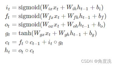
下面计算出来的 temp 在第 1 维(从第 0 维开始计算,例如二维矩阵里,行就是第 0 维,列就是第 1 维)上共有 4h 个特征,要分成四个部分并代入 sigmoid 或 tanh 激活函数进行计算得出 i、f、o、g 。
def lstm_step_forward(x, prev_h, prev_c, Wx, Wh, b):
    """
    Forward pass for a single timestep of an LSTM.

    The input data has dimension D, the hidden state has dimension H, and we use
    a minibatch size of N.

    Inputs:
    - x: Input data, of shape (N, D)
    - prev_h: Previous hidden state, of shape (N, H)
    - prev_c: previous cell state, of shape (N, H)
    - Wx: Input-to-hidden weights, of shape (D, 4H)
    - Wh: Hidden-to-hidden weights, of shape (H, 4H)
    - b: Biases, of shape (4H,)

    Returns a tuple of:
    - next_h: Next hidden state, of shape (N, H)
    - next_c: Next cell state, of shape (N, H)
    - cache: Tuple of values needed for backward pass.
    """
    next_h, next_c, cache = None, None, None
    #############################################################################
    # TODO: Implement the forward pass for a single timestep of an LSTM.        #
    # You may want to use the numerically stable sigmoid implementation above.  #
    #############################################################################
    N, H = prev_h
    temp = np.dot(x, Wx) + np.dot(prev_h, Wh) + b
    #* 将 temp 的 4H 特征分别分给四个门
    i = sigmoid(temp[:, 0:H])
    f = sigmoid(temp[:, H:2*H])
    o = sigmoid(temp[:, 2*H:3*H])
    g = np.tanh(temp[:, 3*H:4*H])
    next_c = f * prev_c + i * g
    next_h = o * np.tanh(next_c)

    cache = (i, f, o, g, x, Wx, Wh, prev_c, prev_h, next_c)
    ##############################################################################
    #                               END OF YOUR CODE                             #
    ##############################################################################

    return next_h, next_c, cache
lstm_step_backward()
tanh激活函数在本篇博文前面有叙述就不再重复,其函数形式和求导结果可移到前面去观看。下面介绍一下 sigmoid 激活函数。
sigmoid激活函数
其函数形式是:
s i g m o i d ( x ) = 1 1 + e − x sigmoid(x) = \frac{1}{1+e^{-x}} sigmoid(x)=1+e−x1该函数对 x 求导的结果是:
s i g m o i d ′ ( x ) = s i g m o i d ∗ ( 1 − s i g m o i d ) sigmoid^{'}(x) = sigmoid * (1 - sigmoid) sigmoid′(x)=sigmoid∗(1−sigmoid)
可以求导一下,最后结果和上式是一样的,但是用上式书写和计算都更加简便。
梯度计算
注意:在前向传播时 t e m p = W x x + W h h + b temp = W_xx + W_hh + b temp=Wxx+Whh+b 被分成四个部分分别来计算 i、f、o、g ,因此在利用 dtemp 来计算 dx、dh、dc、dWx、dWh、db 时要先计算出 i、f、o、g 的梯度,况且使用 di、df、do、dg 计算 dx、dh、dc、dWx、dWh、db 还要注意是一个含有 sigmoid 或 tanh 的复合函数。
下面是 LSTM 前向传播和反向传播的计算图,红色箭头是反向传播的方向。
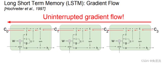
其中 np.hstack() 函数用于在列方向上组合矩阵。
def lstm_step_backward(dnext_h, dnext_c, cache):
    """
    Backward pass for a single timestep of an LSTM.

    Inputs:
    - dnext_h: Gradients of next hidden state, of shape (N, H)
    - dnext_c: Gradients of next cell state, of shape (N, H)
    - cache: Values from the forward pass

    Returns a tuple of:
    - dx: Gradient of input data, of shape (N, D)
    - dprev_h: Gradient of previous hidden state, of shape (N, H)
    - dprev_c: Gradient of previous cell state, of shape (N, H)
    - dWx: Gradient of input-to-hidden weights, of shape (D, 4H)
    - dWh: Gradient of hidden-to-hidden weights, of shape (H, 4H)
    - db: Gradient of biases, of shape (4H,)
    """
    dx, dh, dc, dWx, dWh, db = None, None, None, None, None, None
    #############################################################################
    # TODO: Implement the backward pass for a single timestep of an LSTM.       #
    #                                                                           #
    # HINT: For sigmoid and tanh you can compute local derivatives in terms of  #
    # the output value from the nonlinearity.                                   #
    #############################################################################
    i, f, o, g, x, Wx, Wh, prev_c, prev_h, next_c = cache
    do = dnext_h * np.tanh(next_c)
    dnext_c += dnext_h * o * (1 - np.tanh(next_c)**2)
    di = dnext_c * g
    dg = dnext_c * i
    dprev_c = dnext_c * f
    df = dnext_c * prev_c
    #! d(sigmoid) = sigmoid * (1 - sigmoid)
    #! d(tanh) = 1 - tanh^2
    dtemp = np.hstack([di * i * (1 - i), df * f * (1 - f), do * o * (1 - o), dg * (1 - g**2)])
    dx = np.dot(dtemp, Wx.T)
    dprev_h = np.dot(dtemp, Wh.T)
    dWx = np.dot(x.T, dtemp)
    dWh = np.dot(prev_h.T, dtemp)
    db = np.sum(dtemp, 0)
    ##############################################################################
    #                               END OF YOUR CODE                             #
    ##############################################################################

    return dx, dprev_h, dprev_c, dWx, dWh, db
lstm_forward()
这个函数是 LSTM 的总体前向传播的函数,输入 x 加入了时间维度,需要嵌套调用lstm_step_forward() 函数。其输出 h 是一个数组,记录了 LSTM 网络每个时刻的状态。我们使用 for 循环模拟时间的推移,因此在数组 h 中存储的维度是 [T, N, H] ,这不是我们想要的维度顺序,因此使用 transpose() 函数来变换维度顺序。
def lstm_forward(x, h0, Wx, Wh, b):
    """
    Forward pass for an LSTM over an entire sequence of data. We assume an input
    sequence composed of T vectors, each of dimension D. The LSTM uses a hidden
    size of H, and we work over a minibatch containing N sequences. After running
    the LSTM forward, we return the hidden states for all timesteps.

    Note that the initial cell state is passed as input, but the initial cell
    state is set to zero. Also note that the cell state is not returned; it is
    an internal variable to the LSTM and is not accessed from outside.

    Inputs:
    - x: Input data of shape (N, T, D)
    - h0: Initial hidden state of shape (N, H)
    - Wx: Weights for input-to-hidden connections, of shape (D, 4H)
    - Wh: Weights for hidden-to-hidden connections, of shape (H, 4H)
    - b: Biases of shape (4H,)

    Returns a tuple of:
    - h: Hidden states for all timesteps of all sequences, of shape (N, T, H)
    - cache: Values needed for the backward pass.
    """
    h, cache = None, None
    #############################################################################
    # TODO: Implement the forward pass for an LSTM over an entire timeseries.   #
    # You should use the lstm_step_forward function that you just defined.      #
    #############################################################################
    T = x.shape[1]
    prev_h = h0
    prev_c = np.zeros_like(h0) #* c 是(N, H)的维度
    h, cache = [], []
    for t in range(T):
        next_h, next_c, temp_cache = lstm_step_forward(x[:, t, :], prev_h, prev_c, Wx, Wh, b)
        cache.append(temp_cache)
        h.append(next_h)
        prev_h = next_h
        prev_c = next_c
    h = np.array(h).transpose(1, 0, 2)
    ##############################################################################
    #                               END OF YOUR CODE                             #
    ##############################################################################

    return h, cache
lstm_backward()
其中的步骤和 rnn_backward() 差不多,要注意的也是在调用 lstm_step_backward() 函数时传入的 dnext_h 参数。dnext_h 是需要叠加从上面(也就是h,即总体的状态的梯度)和右边(next_h)传来的梯度,而不是单纯只传入下一个状态(next_h)的梯度,当前时刻的状态有参与到所有状态的梯度的计算中,体现在dh[:, t, :],也有传播到下一个状态next_h,再计算下一个状态的损失,所以要叠加h的和next_h的梯度
def lstm_backward(dh, cache):
    """
    Backward pass for an LSTM over an entire sequence of data.]

    Inputs:
    - dh: Upstream gradients of hidden states, of shape (N, T, H)
    - cache: Values from the forward pass

    Returns a tuple of:
    - dx: Gradient of input data of shape (N, T, D)
    - dh0: Gradient of initial hidden state of shape (N, H)
    - dWx: Gradient of input-to-hidden weight matrix of shape (D, 4H)
    - dWh: Gradient of hidden-to-hidden weight matrix of shape (H, 4H)
    - db: Gradient of biases, of shape (4H,)
    """
    dx, dh0, dWx, dWh, db = None, None, None, None, None
    #############################################################################
    # TODO: Implement the backward pass for an LSTM over an entire timeseries.  #
    # You should use the lstm_step_backward function that you just defined.     #
    #############################################################################
    N, T, H = dh.shape
    D = cache[0][4].shape[1]
    ddh = np.zeros((N, H))
    ddc = np.zeros((N, H))
    dx = []
    dWx = np.zeros((N, 4*H))
    dWh = np.zeros((H, 4*H))
    db = np.zeros(4*H)
    for t in range(T - 1, -1, -1):
        ddx, ddh, ddc, ddWx, ddWh, ddb = lstm_step_backward(dh[:, t, :] + ddh, ddc, cache[t])
        dx.append(ddx)
        dWx = dWx + ddWx
        dWh = dWh + ddWh
        db = db + ddb
    dh0 = ddh
    dx = np.array(dx[::-1]).transpose(1, 0, 2)
    ##############################################################################
    #                               END OF YOUR CODE                             #
    ##############################################################################

    return dx, dh0, dWx, dWh, db
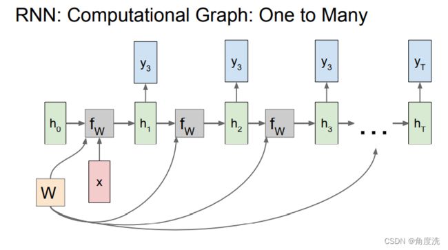
RNN、LSTM 网络示意图对比总结

RNN_Captioning.ipynb
这一个文件是需要我们运行观察结果的文件,里面没有需要写的代码。可以到我的GitHub仓库看运行结果。
LSTM_Captioning.ipynb
这一部分所需要用到的 LSTM 的函数在 rnn_layers.py 的部分中已经讲解完毕,可以移到上面去查看。这一文件中运行的结果可以到我的GitHub仓库查看。
net_visualization_pytorch.py
在这一部分我选择完成 pytorch 版本的,虽然 tensorflow 的出现时间更长,但是近几年 pytorch 的使用趋势急速增长,科研中使用 pytorch 也会更多些。
这一部分我使用的是2020版本的作业,由于我对pytorch不熟,实现上参考了这篇博文:2020 cs231n 作业3 笔记 NetworkVisualization-PyTorch
compute_saliency_maps()
saliency map介绍
saliency map可以理解为特征图,为了衡量图像中每个像素点的特征对分类结果的影响,可以先看一下这一部分运行出的结果,下面一排就是上面一排的 saliency map 。

saliency map实现
- 对输入 X 进行预测类别,得到分类结果 y_pred
- 计算损失 loss
- 求出输入 X 的梯度,取其在RGB 三个通道上的最大值的绝对值
def compute_saliency_maps(X, y, model):
    """
    Compute a class saliency map using the model for images X and labels y.

    Input:
    - X: Input images; Tensor of shape (N, 3, H, W)
    - y: Labels for X; LongTensor of shape (N,)
    - model: A pretrained CNN that will be used to compute the saliency map.

    Returns:
    - saliency: A Tensor of shape (N, H, W) giving the saliency maps for the input
    images.
    """
    # Make sure the model is in "test" mode
    model.eval()

    # Make input tensor require gradient
    X.requires_grad_()

    saliency = None
    ##############################################################################
    # TODO: Implement this function. Perform a forward and backward pass through #
    # the model to compute the gradient of the correct class score with respect  #
    # to each input image. You first want to compute the loss over the correct   #
    # scores (we'll combine losses across a batch by summing), and then compute  #
    # the gradients with a backward pass.                                        #
    ##############################################################################
    # *****START OF YOUR CODE (DO NOT DELETE/MODIFY THIS LINE)*****

    X.requires_grad_(True)
    model.zero_grad()
    loss_fun = torch.nn.CrossEntropyLoss()
    y_pred = model(X)
    loss = loss_fun(y_pred, y)
    loss.requires_grad_(True)
    loss.backward()
    saliency,_ = X.grad.abs().max(axis=1)

    # *****END OF YOUR CODE (DO NOT DELETE/MODIFY THIS LINE)*****
    ##############################################################################
    #                             END OF YOUR CODE                               #
    ##############################################################################
    return saliency
make_fooling_image()
函数目标
这一部分主要是要实现对于输入的图片 X ,给定目标类别 target_y ,输出和 X 很像的 X_fooling 使得 X_fooling 在目标类别上的得分最高(即 loss 最低)。
实现思路
在实现上可以简要的概括为:初始化 X_fooling = X.clone() ,然后对 X_fooling 进行梯度下降使其在 target_y 上得分最高。
注意:在官方给出的函数说明中,在计算更新步长时,首先对梯度进行归一化,公式如下:
u p d a t e _ s t e p = l e a r n i n g _ r a t e ∗ d x ∥ d x ∥ 2 update\_step = \frac{learning\_rate * dx}{\|dx\|^2} update_step=∥dx∥2learning_rate∗dx
def make_fooling_image(X, target_y, model):
    """
    Generate a fooling image that is close to X, but that the model classifies
    as target_y.

    Inputs:
    - X: Input image; Tensor of shape (1, 3, 224, 224)
    - target_y: An integer in the range [0, 1000)
    - model: A pretrained CNN

    Returns:
    - X_fooling: An image that is close to X, but that is classifed as target_y
    by the model.
    """
    # Initialize our fooling image to the input image, and make it require gradient
    X_fooling = X.clone()
    X_fooling = X_fooling.requires_grad_()

    learning_rate = 1
    ##############################################################################
    # TODO: Generate a fooling image X_fooling that the model will classify as   #
    # the class target_y. You should perform gradient ascent on the score of the #
    # target class, stopping when the model is fooled.                           #
    # When computing an update step, first normalize the gradient:               #
    #   dX = learning_rate * g / ||g||_2                                         #
    #                                                                            #
    # You should write a training loop.                                          #
    #                                                                            #
    # HINT: For most examples, you should be able to generate a fooling image    #
    # in fewer than 100 iterations of gradient ascent.                           #
    # You can print your progress over iterations to check your algorithm.       #
    ##############################################################################
    # *****START OF YOUR CODE (DO NOT DELETE/MODIFY THIS LINE)*****

    model.eval()
    X_fooling.requires_grad_()
    iters = 100
    y = torch.LongTensor([target_y])
    loss_fun = torch.nn.CrossEntropyLoss()
    for i in range(iters):
        print("第" + str(i) + "次迭代")
        score = model(X_fooling)
        print("score", score.argmax(axis = 1)) #* 输出分数最高的类
        print('y', y) #* 输出真实类
        if score.argmax(axis = 1) == y:
            break
        loss = loss_fun(score, y)
        loss.requires_grad_()
        model.zero_grad()
        loss.backward()
        with torch.no_grad():
            g = X_fooling.grad
            dX_fooling = learning_rate * g / torch.norm(g)
            X_fooling -= dX_fooling

    # *****END OF YOUR CODE (DO NOT DELETE/MODIFY THIS LINE)*****
    ##############################################################################
    #                             END OF YOUR CODE                               #
    ##############################################################################
    return X_fooling
class_visualization_update_step()
函数作用
给出图片 img 和目标分类 targe_y ,对 img 进行梯度上升从而增加 img 在目标类别上的得分。
实现细节
由于需要让目标类别的分数最高,因此我们不是像之前用 loss 来对参数求梯度,再使用梯度下降来降低 loss ,而是使用目标类别的分数 sy 对参数求梯度,再使用梯度上升。
区别就在于计算了分数之后,为了使得分数更高就用了梯度上升,之前是计算loss,为了使loss更低所以用了梯度下降
还要注意一点是官方的函数实现说明中写明梯度上升步长是 img 的梯度以及 img 的 L2 正则项。
def class_visualization_update_step(img, model, target_y, l2_reg, learning_rate):
    ########################################################################
    # TODO: Use the model to compute the gradient of the score for the     #
    # class target_y with respect to the pixels of the image, and make a   #
    # gradient step on the image using the learning rate. Don't forget the #
    # L2 regularization term!                                              #
    # Be very careful about the signs of elements in your code.            #
    ########################################################################
    # *****START OF YOUR CODE (DO NOT DELETE/MODIFY THIS LINE)*****

    model.eval()
    img.requires_grad_()
    score = model(img)
    sy = score[:, target_y] #! 取出每个样本在目标类别上的得分
    sy.requires_grad_()
    model.zero_grad()
    sy.backward()
    dimg = img.grad + 2 * l2_reg * img #! 加上正则项
    with torch.no_grad():
        dimg /= torch.norm(dimg)
        img += learning_rate * dimg #! 由于是要让在目标类别上的得分最高,使用的是梯度上升,所以是 += 的符号

    # *****END OF YOUR CODE (DO NOT DELETE/MODIFY THIS LINE)*****
    ########################################################################
    #                             END OF YOUR CODE                         #
    ########################################################################
NetworkVisualization.ipynb
这一个文件是需要我们运行观察结果的文件,里面没有需要写的代码。可以到我的GitHub仓库看。
StyleTransfer-PyTorch.ipynb
这一个文件是用来实现风格转换的,我选择的pytorch版本来实现,主要参考的是2020 cs231n 作业3 笔记 StyleTransfer-PyTorch,里面运行结果可以到我的GitHub仓库看。
这一部分的损失函数 loss 主要由下面三个部分组成:content loss + style loss + total variation loss
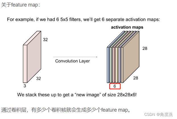
content_loss()
这个函数是用于计算原图片和生成的图片之间像素的差距,使用的是之前定义的 extract_features() 函数提取的卷积层获取的 feature map 的特征进行差距的计算。参考上面提到的博文中对于 feature map 的一段解释:
content loss 的计算公式是: L c = w c × ∑ i , j ( F i j ℓ − P i j ℓ ) 2 L_c = w_c \times \sum_{i,j} (F_{ij}^{\ell} - P_{ij}^{\ell})^2 Lc=wc×i,j∑(Fijℓ−Pijℓ)2其中 w c w_c wc 是损失权重, ℓ \ell ℓ 是通道层,对于 content loss 所有的通道都要参与激素, F F F 是生成的图片, P P P 是原来的图片。
给出的输入参数有:content_loss:是损失权重,即 W c W_c Wccontent_current 是生成的图片,即 F F F ;content_original 是原图片,即 P P P 。
def content_loss(content_weight, content_current, content_original):
  """
  Compute the content loss for style transfer.

  Inputs:
  - content_weight: Scalar giving the weighting for the content loss.
  - content_current: features of the current image; this is a PyTorch Tensor of shape
    (1, C_l, H_l, W_l).
  - content_target: features of the content image, Tensor with shape (1, C_l, H_l, W_l).

  Returns:
  - scalar content loss
  """
  N, C, H, W = content_current.shape
  Lc = content_weight * (content_current - content_original).pow(2).sum()
  return Lc
gram_matrix()
这一个函数是用来为计算 style_loss 做准备的,需要计算gram矩阵,gram矩阵可以认为是协方差矩阵的近似值,表示的是feature map每个通道(channel)之间的联系(也就是风格)。因为我们希望我们生成的图像的激活统计信息与我们的风格图像的激活统计信息相匹配,匹配(近似)协方差是一种方法,有多种方法可以做到这一点,但 Gram 矩阵很好,因为它易于计算并且在实践中显示出良好的结果。
给定 features (即 feature map ),输入的 features 维度为 ( N , C , H , W ) (N,C,H,W) (N,C,H,W),转换为 ( N , C , M ) (N,C,M) (N,C,M),其中 M = H ∗ W M=H*W M=H∗W,则输出的G维度为 ( N , C , C ) (N,C,C) (N,C,C)。官方给出的计算公式是:
Given a feature map F ℓ F^\ell Fℓ of shape ( 1 , C ℓ , M ℓ ) (1, C_\ell, M_\ell) (1,Cℓ,Mℓ), the Gram matrix has shape ( 1 , C ℓ , C ℓ ) (1, C_\ell, C_\ell) (1,Cℓ,Cℓ) and its elements are given by:
G i j ℓ = ∑ k F i k ℓ F j k ℓ G_{ij}^\ell = \sum_k F^{\ell}_{ik} F^{\ell}_{jk} Gijℓ=k∑FikℓFjkℓ
其中 ℓ \ell ℓ 是表示第几层的 feature map ,其实可以忽略,将维度转换为正确的 ( N , C , M ) (N,C,M) (N,C,M)后使用矩阵乘法自己乘自己就行了。
def gram_matrix(features, normalize=True):
  """
  Compute the Gram matrix from features.

  Inputs:
  - features: PyTorch Variable of shape (N, C, H, W) giving features for
    a batch of N images.
  - normalize: optional, whether to normalize the Gram matrix
      If True, divide the Gram matrix by the number of neurons (H * W * C)

  Returns:
  - gram: PyTorch Variable of shape (N, C, C) giving the
    (optionally normalized) Gram matrices for the N input images.
  """
  #! 计算gram矩阵,具体公式看上面那段介绍中 G_{ij}^l 的那行
  N, C, H, W = features.shape
  F = features.view(N, C, H * W) #! 把后面两个相乘即 H * W 后
  F_t = F.permute(0, 2, 1) #! 计算矩阵 F 的转置
  gram = torch.matmul(F, F_t)
  if normalize:
    gram /= (H * W * C)
  return gram
style_loss()
style loss 的计算公式是:
L s ℓ = w ℓ ∑ i , j ( G i j ℓ − A i j ℓ ) 2 L_s^\ell = w_\ell \sum_{i, j} \left(G^\ell_{ij} - A^\ell_{ij}\right)^2 Lsℓ=wℓi,j∑(Gijℓ−Aijℓ)2
其中: ℓ \ell ℓ 的意义和之前一样,代表第 ℓ \ell ℓ 层的 feature map; G G G 是生成的图片第 ℓ \ell ℓ 层的 feature map 的 gram matrix , A A A 是原来的图片第 ℓ \ell ℓ 层的 feature map 的 gram matrix 。
注意:在实践中,我们通常在一组层 L \mathcal{L} L 而不是单层 ℓ \ell ℓ 上计算样式损失,因此总的风格损失是每一层的风格损失的总和,即总的损失 L s L_s Ls :
L s = ∑ ℓ ∈ L L s ℓ L_s = \sum_{\ell \in \mathcal{L}} L_s^\ell Ls=ℓ∈L∑Lsℓ
# Now put it together in the style_loss function...
def style_loss(feats, style_layers, style_targets, style_weights):
  """
  Computes the style loss at a set of layers.

  Inputs:
  - feats: list of the features at every layer of the current image, as produced by
    the extract_features function.
  - style_layers: List of layer indices into feats giving the layers to include in the
    style loss.
  - style_targets: List of the same length as style_layers, where style_targets[i] is
    a PyTorch Variable giving the Gram matrix the source style image computed at
    layer style_layers[i].
  - style_weights: List of the same length as style_layers, where style_weights[i]
    is a scalar giving the weight for the style loss at layer style_layers[i].

  Returns:
  - style_loss: A PyTorch Variable holding a scalar giving the style loss.
  """
  # Hint: you can do this with one for loop over the style layers, and should
  # not be very much code (~5 lines). You will need to use your gram_matrix function.
  style_current = []
  style_loss = 0
  for i, idx in enumerate(style_layers):
    style_current.append(gram_matrix(feats[idx].clone())) #! 使用 gram matrix 表示的是 feature map 每个通道(channel)之间的联系(也就是风格),可以直接看作风格矩阵,表示第 idx 层的特征列表是从 feats[idx] 取出,根据这个特征列表的特征从风格矩阵中取出这些风格
    style_loss += style_weights[i] * torch.sum((style_current[i] - style_targets[i])**2)
  return style_loss
tv_loss()
为了提高图像的平滑度,使用 tv_loss() 在我们的损失中添加一个项来惩罚像素值的摆动来做到这一点,即去噪。
实现思路:可以计算彼此相邻(水平或垂直)的所有像素对的像素值差的平方和。在这里,我们将 3 个输入通道 (RGB) 中的每一个的总变化正则化相加,并通过总变化权重 w t w_t wt 对总和损失进行加权,具体公式为:
L t v = w t × ∑ c = 1 3 ∑ i = 1 H − 1 ∑ j = 1 W − 1 ( ( x i , j + 1 , c − x i , j , c ) 2 + ( x i + 1 , j , c − x i , j , c ) 2 ) L_{tv} = w_t \times \sum_{c=1}^3\sum_{i=1}^{H-1} \sum_{j=1}^{W-1} \left( (x_{i,j+1, c} - x_{i,j,c})^2 + (x_{i+1, j,c} - x_{i,j,c})^2 \right) Ltv=wt×∑c=13∑i=1H−1∑j=1W−1((xi,j+1,c−xi,j,c)2+(xi+1,j,c−xi,j,c)2)
这里的下标是从 1 开始的,在写代码时要注意从 0 开始。
def tv_loss(img, tv_weight):
  """
  Compute total variation loss.

  Inputs:
  - img: PyTorch Variable of shape (1, 3, H, W) holding an input image.
  - tv_weight: Scalar giving the weight w_t to use for the TV loss.

  Returns:
  - loss: PyTorch Variable holding a scalar giving the total variation loss
    for img weighted by tv_weight.
  """
  # Your implementation should be vectorized and not require any loops!
  #* total variation loss可以使图像变得平滑。信号处理中,总变差去噪,也称为总变差正则化,是最常用于数字图像处理的过程,其在噪声去除中具有应用。
  N, C, H, W = img.shape
  x1 = img[:, :, 0:H-1, :]
  x2 = img[:, :, 1:H, :]
  x3 = img[:, :, :, 0:W-1]
  x4 = img[:, :, :, 1:W]
  loss = tv_weight * ((x4 - x3).pow(2).sum() + (x2 - x1).pow(2).sum())
  return loss
GANs-PyTorch.ipynb / Generative_Adversarial_Networks_PyTorch.ipynb
这一部分主要参考了2020 cs231n 作业3 笔记 Generative_Adversarial_Networks_PyTorch,里面运行结果可以到我的GitHub仓库看。
GAN网络简单总结
GAN网络由两大部分组成:生成器 Generator 和判别器 Discriminator ,其中生成器尽力生成完美的图片来让判别器把它认成真的,即让得分尽量接近 1 ;而判别器就是尽量判别出我们输入的真图片使其分数尽量接近 1 ,判别出生成器生成的假图片使其分数尽量接近 0,最后就可以使用生成器来生成我们想要的图片。我们的训练目标可以总结成公式如下:(以下为官方解释)
We can think of this back and forth process of the generator ( G G G) trying to fool the discriminator ( D D D), and the discriminator trying to correctly classify real vs. fake as a minimax game:
minimize G maximize D E x ∼ p data [ log D ( x ) ] + E z ∼ p ( z ) [ log ( 1 − D ( G ( z ) ) ) ] \underset{G}{\text{minimize}}\; \underset{D}{\text{maximize}}\; \mathbb{E}_{x \sim p_\text{data}}\left[\log D(x)\right] + \mathbb{E}_{z \sim p(z)}\left[\log \left(1-D(G(z))\right)\right] GminimizeDmaximizeEx∼pdata[logD(x)]+Ez∼p(z)[log(1−D(G(z)))]
我们会让生成器和迭代器来交替更新(免得其中一个拖后腿造成另一个也没法进步,错误的认为当前就是最好的情况),其步骤以及各自的目标函数是:
- 更新generator (G) 以最大化discriminator做出错误分类的概率:
maximize G E z ∼ p ( z ) [ log D ( G ( z ) ) ] \underset{G}{\text{maximize}}\; \mathbb{E}_{z \sim p(z)}\left[\log D(G(z))\right] GmaximizeEz∼p(z)[logD(G(z))] - 更新discriminator (D) 以最大化discriminator做出正确分类的概率:
maximize D E x ∼ p data [ log D ( x ) ] + E z ∼ p ( z ) [ log ( 1 − D ( G ( z ) ) ) ] \underset{D}{\text{maximize}}\; \mathbb{E}_{x \sim p_\text{data}}\left[\log D(x)\right] + \mathbb{E}_{z \sim p(z)}\left[\log \left(1-D(G(z))\right)\right] DmaximizeEx∼pdata[logD(x)]+Ez∼p(z)[log(1−D(G(z)))]
总结GAN的训练算法
在每一个训练迭代期,我们都要先训练判别器网络然后才是生成器网络,对于判别器网络的 k 个训练步我们将会从噪声先验分布 z 中采样得到一个小批量样本, 接着同样从训练数据 x 中采样获得小批量的真实样本,然后将噪声样本传给生成器网络,并在生成器的输出端获得伪造图像,也就是我们有一个小批量的伪造图像和小批量的真实图像,然后我们会用这些真假小批量数据在判别器上进行一次梯度计算,接下来利用梯度信息更新判别器参数,按照这样的步骤迭代一定次数来训练一会判别器。在这之后执行第二步也就是训练生成器,在这一步我们会采样得到一个小批量的噪声样本把他传入生成器,然后对生成器进行梯度计算,从而优化其目标函数。要交替执行上述两个步骤,也就是交替地在生成器和判别器上计算梯度,要努力平衡两个网络。
sample_noise()
由于生成器G是从以噪声为初始数据来生成图片,因此这个函数是用来生成随机噪音作为G的初始数据的。需要生成 [-1, 1] 之间shape为 [batch_size, dim] 的数据。
def sample_noise(batch_size, dim):
  """
  Generate a PyTorch Tensor of uniform random noise.

  Input:
  - batch_size: Integer giving the batch size of noise to generate.
  - dim: Integer giving the dimension of noise to generate.

  Output:
  - A PyTorch Tensor of shape (batch_size, dim) containing uniform
    random noise in the range (-1, 1).
  """
  ##############################################################################
  # TODO: Implement architecture                                               #
  #                                                                            #
  # HINT: nn.Sequential might be helpful.                                      #
  ##############################################################################
  # *****START OF YOUR CODE (DO NOT DELETE/MODIFY THIS LINE)*****

  #* 注意生成器G是以噪声为初始数据来生成图片的
  out = torch.rand(batch_size, dim)
  out = 2 * out - 1 #! 限定输出随机数的范围是 [-1, 1]
  return out

  # *****END OF YOUR CODE (DO NOT DELETE/MODIFY THIS LINE)*****
  ##############################################################################
  #                               END OF YOUR CODE                             #
  ##############################################################################
discriminator()
判别器D的网络结构是:
- Fully connected layer from size 784 to 256
- LeakyReLU with alpha 0.01
- Fully connected layer from 256 to 256
- LeakyReLU with alpha 0.01
- Fully connected layer from 256 to 1
def discriminator():
    """
    Build and return a PyTorch model implementing the architecture above.
    """
    model = nn.Sequential(
        ##############################################################################
        # TODO: Implement architecture                                               #
        #                                                                            #
        # HINT: nn.Sequential might be helpful.                                      #
        ##############################################################################
        # *****START OF YOUR CODE (DO NOT DELETE/MODIFY THIS LINE)*****

        Flatten(),
        nn.Linear(784, 256),
        nn.LeakyReLU(0.01),
        nn.Linear(256, 256),
        nn.LeakyReLU(0.01),
        nn.Linear(256, 1),

        # *****END OF YOUR CODE (DO NOT DELETE/MODIFY THIS LINE)*****
        ##############################################################################
        #                               END OF YOUR CODE                             #
        ##############################################################################
    )
    return model
generator()
生成器G的网络结构是:
- Fully connected layer from noise_dim to 1024
- ReLU
- Fully connected layer with size 1024
- ReLU
- Fully connected layer with size 784
- TanH (To clip the image to be [-1,1])
def generator(noise_dim=NOISE_DIM):
    """
    Build and return a PyTorch model implementing the architecture above.
    """
    model = nn.Sequential(
        ##############################################################################
        # TODO: Implement architecture                                               #
        #                                                                            #
        # HINT: nn.Sequential might be helpful.                                      #
        ##############################################################################
        # *****START OF YOUR CODE (DO NOT DELETE/MODIFY THIS LINE)*****

        nn.Linear(noise_dim, 1024),
        nn.ReLU(),
        nn.Linear(1024, 1024),
        nn.ReLU(),
        nn.Linear(1024, 784),
        nn.Tanh(),

        # *****END OF YOUR CODE (DO NOT DELETE/MODIFY THIS LINE)*****
        ##############################################################################
        #                               END OF YOUR CODE                             #
        ##############################################################################
    )
    return model
bce_loss()
使用 bce_loss 函数来计算二进制交叉熵损失,这是在给定预测输出后计算其预测损失的函数,用在判别器D和生成器G中。给定分数 s ∈ R s\in\mathbb{R} s∈R 和标签 y ∈ { 0 , 1 } y\in\{0, 1\} y∈{0,1},二元交叉熵损失为: b c e ( s , y ) = y ∗ log ( s ) + ( 1 − y ) ∗ log ( 1 − s ) bce(s, y) = y * \log(s) + (1 - y) * \log(1 - s) bce(s,y)=y∗log(s)+(1−y)∗log(1−s)
def bce_loss(input, target):
    """
    Numerically stable version of the binary cross-entropy loss function.

    As per https://github.com/pytorch/pytorch/issues/751
    See the TensorFlow docs for a derivation of this formula:
    https://www.tensorflow.org/api_docs/python/tf/nn/sigmoid_cross_entropy_with_logits

    Inputs:
    - input: PyTorch Variable of shape (N, ) giving scores.
    - target: PyTorch Variable of shape (N,) containing 0 and 1 giving targets.

    Returns:
    - A PyTorch Variable containing the mean BCE loss over the minibatch of input data.
    """
    neg_abs = - input.abs()
    loss = input.clamp(min=0) - input * target + (1 + neg_abs.exp()).log()
    return loss.mean()
discriminator_loss()
判别器D的损失计算公式定义如下:
ℓ D = − E x ∼ p data [ log D ( x ) ] − E z ∼ p ( z ) [ log ( 1 − D ( G ( z ) ) ) ] \ell_D = -\mathbb{E}_{x \sim p_\text{data}}\left[\log D(x)\right] - \mathbb{E}_{z \sim p(z)}\left[\log \left(1-D(G(z))\right)\right] ℓD=−Ex∼pdata[logD(x)]−Ez∼p(z)[log(1−D(G(z)))]
其中 x x x 是我们输入的真实图片, z z z 是初始的假图片, G ( z ) G(z) G(z) 是生成器生成的假图片, D ( ) D() D() 是判别器D对真假图片进行判别后的分数。
def discriminator_loss(logits_real, logits_fake):
    """
    Computes the discriminator loss described above.

    Inputs:
    - logits_real: PyTorch Variable of shape (N,) giving scores for the real data.
    - logits_fake: PyTorch Variable of shape (N,) giving scores for the fake data.

    Returns:
    - loss: PyTorch Variable containing (scalar) the loss for the discriminator.
    """

    # *****START OF YOUR CODE (DO NOT DELETE/MODIFY THIS LINE)*****

    real = torch.ones_like(logits_real).type(dtype) #! 对于真数据的理想标签应该是 1
    fake = torch.zeros_like(logits_fake).type(dtype) #! 对于假数据的理想标签应该是 0
    real_loss = bce_loss(logits_real, real) #! 判别器判断真数据时的 loss
    fake_loss = bce_loss(logits_fake, fake) #! 判别器判断假数据时的 loss
    loss = real_loss + fake_loss

    # *****END OF YOUR CODE (DO NOT DELETE/MODIFY THIS LINE)*****

    return loss
generator_loss()
生成器G的损失计算公式为: ℓ G = − E z ∼ p ( z ) [ log D ( G ( z ) ) ] \ell_G = -\mathbb{E}_{z \sim p(z)}\left[\log D(G(z))\right] ℓG=−Ez∼p(z)[logD(G(z))]其中 z z z 是初始的假图片, G ( z ) G(z) G(z) 是生成器生成的假图片, D ( ) D() D() 是判别器D对真假图片进行判别后的分数。
def generator_loss(logits_fake):
    """
    Computes the generator loss described above.

    Inputs:
    - logits_fake: PyTorch Variable of shape (N,) giving scores for the fake data.

    Returns:
    - loss: PyTorch Variable containing the (scalar) loss for the generator.
    """

    # *****START OF YOUR CODE (DO NOT DELETE/MODIFY THIS LINE)*****

    fake = torch.ones_like(logits_fake).type(dtype) #! 全 1 目标分数矩阵,用于计算损失
    loss = bce_loss(logits_fake, fake) #! 生成器的损失定义为判别器给出生成器生成的假图片的分数与 1 的差距,其中 1 是判别器给出百分之百确定是真实图片的分数

    # *****END OF YOUR CODE (DO NOT DELETE/MODIFY THIS LINE)*****

    return loss
get_optimizer()
这个函数用来定义优化器,使用的是Adam优化算法。
def get_optimizer(model):
    """
    Construct and return an Adam optimizer for the model with learning rate 1e-3,
    beta1=0.5, and beta2=0.999.

    Input:
    - model: A PyTorch model that we want to optimize.

    Returns:
    - An Adam optimizer for the model with the desired hyperparameters.
    """
    # *****START OF YOUR CODE (DO NOT DELETE/MODIFY THIS LINE)*****

    optimizer = optim.Adam(model.parameters(), lr=1e-3, betas=(0.5, 0.999))

    # *****END OF YOUR CODE (DO NOT DELETE/MODIFY THIS LINE)*****
    return optimizer
ls_discriminator_loss()
Least Squares GAN 是使用另一种计算 GAN 的损失的计算方法。它是原始 GAN 损失函数的更新、更稳定的替代方案,对于这一部分,我们所要做的就是改变损失函数并重新训练模型。
判别器D的损失计算定义如下:
ℓ D = 1 2 E x ∼ p data [ ( D ( x ) − 1 ) 2 ] + 1 2 E z ∼ p ( z ) [ ( D ( G ( z ) ) ) 2 ] \ell_D = \frac{1}{2}\mathbb{E}_{x \sim p_\text{data}}\left[\left(D(x)-1\right)^2\right] + \frac{1}{2}\mathbb{E}_{z \sim p(z)}\left[ \left(D(G(z))\right)^2\right] ℓD=21Ex∼pdata[(D(x)−1)2]+21Ez∼p(z)[(D(G(z)))2]
def ls_discriminator_loss(scores_real, scores_fake):
    """
    Compute the Least-Squares GAN loss for the discriminator.

    Inputs:
    - scores_real: PyTorch Variable of shape (N,) giving scores for the real data.
    - scores_fake: PyTorch Variable of shape (N,) giving scores for the fake data.

    Outputs:
    - loss: A PyTorch Variable containing the loss.
    """
    # *****START OF YOUR CODE (DO NOT DELETE/MODIFY THIS LINE)*****

    real_loss = 0.5 * (scores_real - 1).pow(2)
    fake_loss = 0.5 * scores_fake.pow(2)
    real_loss = real_loss.mean()
    fake_loss = fake_loss.mean()
    loss = real_loss + fake_loss

    # *****END OF YOUR CODE (DO NOT DELETE/MODIFY THIS LINE)*****

    return loss
ls_generator_loss()
生成器G的损失计算定义如下:
ℓ G = 1 2 E z ∼ p ( z ) [ ( D ( G ( z ) ) − 1 ) 2 ] \ell_G = \frac{1}{2}\mathbb{E}_{z \sim p(z)}\left[\left(D(G(z))-1\right)^2\right] ℓG=21Ez∼p(z)[(D(G(z))−1)2]
def ls_generator_loss(scores_fake):
    """
    Computes the Least-Squares GAN loss for the generator.

    Inputs:
    - scores_fake: PyTorch Variable of shape (N,) giving scores for the fake data.

    Outputs:
    - loss: A PyTorch Variable containing the loss.
    """
    # *****START OF YOUR CODE (DO NOT DELETE/MODIFY THIS LINE)*****

    loss = 0.5 * (scores_fake - 1).pow(2)
    loss = loss.mean()

    # *****END OF YOUR CODE (DO NOT DELETE/MODIFY THIS LINE)*****
    return loss
build_dc_classifiebuild_dc_classifier()
这一部分我们实现的是 Deeply Convolutional GANs ,在之前的部分中,我们实现了 Ian Goodfellow 原始 GAN 网络。然而,这种网络架构不允许真正的空间推理。它通常无法推理诸如“锐边”之类的东西,因为它缺少任何卷积层。因此,在本节中,我们将实现 DCGAN 中的一些想法,即实现深度卷积GAN。
我们将使用受 TensorFlow MNIST 分类教程启发的判别器,它能够相当快地在 MNIST 数据集上达到 99% 以上的准确率。判别器D的网络结构定义为:
- Reshape into image tensor (Use Unflatten!)
- 32 Filters, 5x5, Stride 1, Leaky ReLU(alpha=0.01)
- Max Pool 2x2, Stride 2
- 64 Filters, 5x5, Stride 1, Leaky ReLU(alpha=0.01)
- Max Pool 2x2, Stride 2
- Flatten
- Fully Connected size 4 x 4 x 64, Leaky ReLU(alpha=0.01)
- Fully Connected size 1
def build_dc_classifier(batch_size):
    """
    Build and return a PyTorch model for the DCGAN discriminator implementing
    the architecture above.
    """
    return nn.Sequential(

        Unflatten(batch_size, 1, 28, 28),
        ###########################
        ######### TO DO ###########
        nn.Conv2d(1, 32, 5),
        nn.LeakyReLU(0.01),
        nn.MaxPool2d(2,2),
        nn.Conv2d(32, 64, 5),
        nn.LeakyReLU(0.01),
        nn.MaxPool2d(2,2),
        Flatten(),
        nn.Linear(64*4*4, 4*4*64),
        nn.LeakyReLU(0.01),
        nn.Linear(64*4*4, 1),
        ###########################

    )
build_dc_generator()
生成器G的网络结构定义为:
- Fully connected with output size 1024
ReLU- BatchNorm
- Fully connected with output size 7 x 7 x 128
- ReLU
- BatchNorm
- Reshape into Image Tensor of shape 7, 7, 128
- Conv2D^T (Transpose): 64 filters of 4x4, stride 2, ‘same’ padding (use
padding=1) ReLU- BatchNorm
- Conv2D^T (Transpose): 1 filter of 4x4, stride 2, ‘same’ padding (use
padding=1) TanH- Should have a 28x28x1 image, reshape back into 784 vector
def build_dc_generator(noise_dim=NOISE_DIM):
    """
    Build and return a PyTorch model implementing the DCGAN generator using
    the architecture described above.
    """
    return nn.Sequential(
        ###########################
        ######### TO DO ###########
        nn.Linear(noise_dim, 1024),
        nn.ReLU(),
        nn.BatchNorm1d(1024), #* 里面那个参数是特征维度
        nn.Linear(1024, 7*7*128),
        nn.ReLU(),
        nn.BatchNorm1d(7*7*128),
        Unflatten(-1, 128, 7, 7),
        nn.ConvTranspose2d(128, 64, kernel_size=4, stride=2, padding=1), #! https://zhuanlan.zhihu.com/p/48501100 上采样方法之一————反卷积的介绍
        nn.ReLU(),
        nn.BatchNorm2d(64),
        nn.ConvTranspose2d(64, 1, kernel_size=4, stride=2, padding=1),
        nn.Tanh(),
        Flatten(),

        ###########################
    )