经典CNN(二）：ResNet50V2算法实战与解析

• 本文为365天深度学习训练营中的学习记录博客
• 原作者：K同学啊|接辅导、项目定制

 1 论文解读

    在《Identity Mappings in Deep Residual Networks》中，作者何凯明先生提出了一种新的残差单元，为区别原始的ResNet结构，这里称其为ResNetV2。

1.1 ResNetV2 & ResNet之结构对比和性能对比

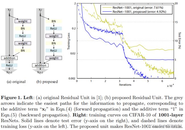
    上图为原始论文中的截图，展示了ResNet和ResNetV2的结构对比，以及测试结果。根据说明可知，右图的实线表示测试误差，对应右边y轴的Test Error，虚线表示训练损失，对应左边y轴的Train Loss，x轴表示迭代次数Iterations。

• 结构调整点：ResNet（图a中的original）结构是(卷积+BN+激活+卷积+BN)+addition+激活，而ResNetV2（图b中的proposed）结构是(BN+激活+卷积+BN+激活+卷积)+addition。对比发现，两者的总模块数和类型未发生改变，只是在顺序上做了调整。
• 结果提升：作者使用两种不同的结构在CIFAR-10数据集上做测试，模型使用1001层的RestNet模型，从右图结果可以看出，ResNetV2的测试集错误率(4.92%)明显低于原始的ResNet(7.61%)。loss方面，同一个Iteration上，ResNetV2都低于ResNet。

1.2 残差的不同尝试

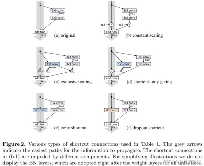
    上图是论文中作者对残差结构的shortcut部分进行的不同尝试，从图示说明中得知，为简化插图，我们不显示BN层，图中所有的conv层之后都有BN层。其测试结果如下表所示，该表是使用ResNet-110在CIFAR-10测试集上的分类错误，对所有残差单元应用了不同类型的shortcut connections，当测试误差大于20%时，标注为“fail”。测试结果表明，原始的ResNet结构是最好的，即恒等映射是最好的。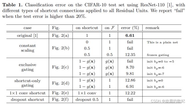

 1.3 激活的不同尝试

     使用不同的激活函数进行尝试，由此可见，最好的结果是full pre-activation，其次是original。

2 代码实现

2.1 开发环境

电脑系统：ubuntu16.04

编译器：Jupter Lab

语言环境：Python 3.7

深度学习环境：tensorflow

2.2 数据准备代码

    这部分代码包括设置GPU和数据处理部分，其中数据处理包括导入数据、查看数据、加载数据、可视化数据、检查数据、配置数据。

2.2.1 设置GPU

import tensorflow as tf

gpus = tf.config.list_physical_devices("GPU")

if gpus:
    tf.config.experimental.set_memory_growth(gpus[0], True) # 设置GPU显存用量按需使用
    tf.config.set_visible_devices([gpus[0]], "GPU")

2.2.2 导入数据

import matplotlib.pyplot as plt
# 支持中文
plt.rcParams['font.sans-serif'] = ['SimHei'] # 用来正常显示中文标签
plt.rcParams['axes.unicode_minus'] = False # 用来正常显示负号

import os, PIL, pathlib
import numpy as np

from tensorflow import keras
from tensorflow.keras import layers,models

data_dir = "../data/bird_photos"
data_dir = pathlib.Path(data_dir)

image_count = len(list(data_dir.glob('*/*')))
print("图片总数为：", image_count)

2.2.3 加载数据

batch_size = 8
img_height = 224
img_width = 224

train_ds = tf.keras.preprocessing.image_dataset_from_directory(
    data_dir,
    validation_split=0.2,
    subset="training",
    seed=123,
    image_size=(img_height, img_width),
    batch_size=batch_size)

val_ds = tf.keras.preprocessing.image_dataset_from_directory(
    data_dir,
    validation_split=0.2,
    subset="validation",
    seed=123,
    image_size=(img_height, img_width),
    batch_size=batch_size)

class_Names = train_ds.class_names
print("class_Names:",class_Names)

    输出结果如下：

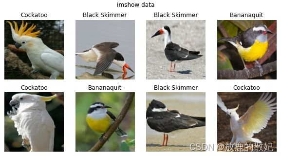
2.2.4 可视化数据

plt.figure(figsize=(10, 5)) # 图形的宽为10，高为5
plt.suptitle("imshow data")

for images,labels in train_ds.take(1):
    for i in range(8):
        ax = plt.subplot(2, 4, i+1)
        plt.imshow(images[i].numpy().astype("uint8"))
        plt.title(class_Names[labels[i]])
        plt.axis("off")

    输出结果如下：

2.2.5 检查数据

for image_batch, lables_batch in train_ds:
    print(image_batch.shape)
    print(lables_batch.shape)
    break

    输出结果如下：

2.2.6 配置数据集

AUTOTUNE = tf.data.AUTOTUNE

train_ds = train_ds.cache().shuffle(1000).prefetch(buffer_size=AUTOTUNE)
val_ds = val_ds.cache().prefetch(buffer_size=AUTOTUNE)

2.3 ResNet50V2模型复现

2.3.1 ResNet50V2网络结构

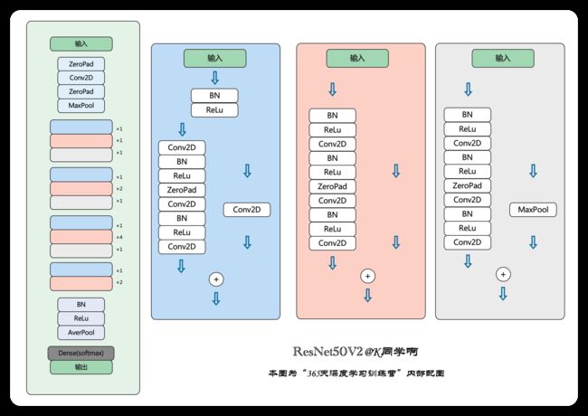
    如下所示，最左边是ResNet50V2的网络结构，与ResNet50类似，但又比ResNet更复杂一点，包括了三个基本的Residual block，分别用蓝色、橙色、灰色块表示。右边是这三个Residual block的网络结构。仔细查看可以得出，三个Residual block左边的分支模块和顺序完全一样，分别为(BN+ReLu)+(Conv2D+BN+ReLU)+ZeroPad+(Conv2D+BN+ReLU)+Conv2D，右边分支有所差异，因此在编写代码的时候，可以共用一个函数，根据传入参数的不同而产生相应的Residual block。

 2.3.2 ResNetV2代码

import tensorflow as tf
import tensorflow.keras.layers as layers
from tensorflow.keras.models import Model


''' 残差块
Arguments:
    x: 输入张量
    filters: integer, filters, of the bottleneck layer.
    kernel_size: default 3, kernel size of the bottleneck layer.
    stride: default 1, stride of the first layer.
    conv_shortcut: default False, use convolution shortcut if True, otherwise identity shortcut.
    name: string, block label.
Returns:
    Output tensor for the residual block.
'''
def block2(x, filters, kernel_size=3, stride=1, conv_shortcut=False, name=None):
    preact = layers.BatchNormalization(name=name+'_preact_bn')(x)
    preact = layers.Activation('relu', name=name+'_preact_relu')(preact)
    
    if conv_shortcut:
        shortcut = layers.Conv2D(4*filters, 1, strides=stride, name=name+'_0_conv')(preact)
    else:
        shortcut = layers.MaxPooling2D(1, strides=stride)(x) if stride>1 else x
    
    x = layers.Conv2D(filters, 1, strides=1, use_bias=False, name=name+'_1_conv')(preact)
    x = layers.BatchNormalization(name=name+'_1_bn')(x)
    x = layers.Activation('relu', name=name+'_1_relu')(x)
    
    x = layers.ZeroPadding2D(padding=((1, 1), (1, 1)), name=name+'_2_pad')(x)
    x = layers.Conv2D(filters, kernel_size, strides=stride, use_bias=False, name=name+'_2_conv')(x)
    x = layers.BatchNormalization(name=name+'_2_bn')(x)
    x = layers.Activation('relu', name=name+'_2_relu')(x)
    
    x = layers.Conv2D(4*filters, 1, name=name+'_3_conv')(x)
    x = layers.Add(name=name+'_out')([shortcut, x])
    return x


def stack2(x, filters, blocks, stride1=2, name=None):
    x = block2(x, filters, conv_shortcut=True, name=name+'_block1')
    for i in range(2, blocks):
        x = block2(x, filters, name=name+'_block'+str(i))
    x = block2(x, filters, stride=stride1, name=name+'_block'+str(blocks))
    return x


''' 构建ResNet50V2 '''
def ResNet50V2(include_top=True,  # 是否包含位于网络顶部的全链接层
               preact=True,  # 是否使用预激活
               use_bias=True,  # 是否对卷积层使用偏置
               weights='imagenet',
               input_tensor=None,  # 可选的keras张量，用作模型的图像输入
               input_shape=None,
               pooling=None,
               classes=1000,  # 用于分类图像的可选类数
               classifer_activation='softmax'):  # 分类层激活函数
    img_input = layers.Input(shape=input_shape)
    x = layers.ZeroPadding2D(padding=((3, 3), (3, 3)), name='conv1_pad')(img_input)
    x = layers.Conv2D(64, 7, strides=2, use_bias=use_bias, name='conv1_conv')(x)
    
    if not preact:
        x = layers.BatchNormalization(name='conv1_bn')(x)
        x = layers.Activation('relu', name='conv1_relu')(x)
    
    x = layers.ZeroPadding2D(padding=((1, 1), (1, 1)), name='pool1_pad')(x)
    x = layers.MaxPooling2D(3, strides=2, name='pool1_pool')(x)
    
    x = stack2(x, 64, 3, name='conv2')
    x = stack2(x, 128, 4, name='conv3')
    x = stack2(x, 256, 6, name='conv4')
    x = stack2(x, 512, 3, stride1=1, name='conv5')
    
    if preact:
        x = layers.BatchNormalization(name='post_bn')(x)
        x = layers.Activation('relu', name='post_relu')(x)
    if include_top:
        x = layers.GlobalAveragePooling2D(name='avg_pool')(x)
        x = layers.Dense(classes, activation=classifer_activation, name='predictions')(x)
    else:
        if pooling=='avg':
            # GlobalAveragePooling2D就是将每张图片的每个通道值各自加起来再求平均，
            # 最后结果是没有了宽高维度，只剩下个数与平均值两个维度
            # 可以理解成变成了多张单像素图片
            x = layers.GlobalAveragePooling2D(name='avg_pool')(x)
        elif pooling=='max':
            x = layers.GlobalMaxPooling2D(name='max_pool')(x)
    
    model = Model(img_input, x, name='resnet50v2')
    return model
    
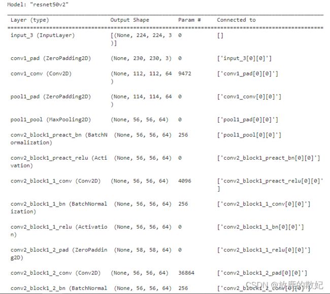
model = ResNet50V2(input_shape=(224,224,3))
model.summary()

    运行结果如下所示（由于输出结果太长，只截取最前面和最后面部分内容）： 

 （中间部分省略）

2.4 设置loss和优化器 

     在对模型进行训练之前，还需要对其设置，包括：

损失函数（loss）：用于衡量模型在训练期间的准确率
优化器（optimizer）：决定模型如何根据其看到的数据和自身的损失函数进行更新。
指标（metrics）：用于监控训练和测试步骤。下面的代码使用了准确率，即被正确分类的图像的比率。

# 设置优化器
opt = tf.keras.optimizers.Adam(learning_rate=1e-7)
 
model.compile(optimizer="adam",
             loss='sparse_categorical_crossentropy',
             metrics=['accuracy'])

2.5 训练模型

epochs = 10
 
history = model.fit(
                train_ds,
                validation_data=val_ds,
                epochs=epochs)

    模型训练时结果：

2.6 模型评估

acc = history.history['accuracy']
val_acc = history.history['val_accuracy']
 
loss = history.history['loss']
val_loss = history.history['val_loss']
 
epochs_range = range(epochs)
 
plt.figure(figsize=(12, 4))
plt.subplot(1, 2, 1)
plt.suptitle("ResNet test")
 
plt.plot(epochs_range, acc, label='Training Accuracy')
plt.plot(epochs_range, val_acc, label='Validation Accuracy')
plt.legend(loc='lower right')
plt.title('Training and Validation Accuracy')
 
plt.subplot(1, 2, 2)
plt.plot(epochs_range, loss, label='Training Loss')
plt.plot(epochs_range, val_loss, label='Validation loss')
plt.legend(loc='upper right')
plt.title('Training and Validation loss')
plt.show()

    结果如图所示：