前言
以下是今天为公司小伙伴们做的ClickHouse技术分享的讲义。由于PPT太难做了,索性直接用Markdown来写,搭配Chrome上的Markdown Preview Plus插件来渲染,效果非常好。
以下全文奉上,浓缩的都是精华,包含之前写过的两篇文章《物化视图简介与ClickHouse中的应用示例》和《ClickHouse Better Practices》中的全部内容,另外也包含一些新内容,如:
- ClickHouse聚合函数的combinator后缀
- 分布式join/in的读放大和GLOBAL关键字
- ClickHouse SQL缺乏开窗分析函数的解决方案
- 示例:排名榜和同比、环比计算
- 以及array join的用法
- LowCardinality数据类型
- MergeTree索引结构
数组和高阶函数没时间说了,之后再提。
开始~
Advanced Usage & Better Practice of ClickHouse
Part I - Materialized View
Intro
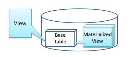
Materialized view (MV): A copy (persistent storage) of query result set
MVs ≠ normal views, but ≈ tables
Space trade-off for time
Exists in various DBMSs (Oracle/SQL Server/PostgreSQL/...)
MV in ClickHouse = Precomputation + Incremental refreshing + Explicit data cache
Usage: Relieve from frequent & patterned aggregating queries
Engines
MaterializedView: Implicit
(Replicated)AggregatingMergeTree: Do auto aggregation upon insertion according to user-defined logic
Distributed: Just like distributed tables before
Creation
- Best-selling merchandise points: PV/UV/first visiting time/last visiting time
【此处图片涉及业务数据,故删掉】
CREATE MATERIALIZED VIEW IF NOT EXISTS dw.merchandise_point_pvuv_agg
ON CLUSTER sht_ck_cluster_1
ENGINE = ReplicatedAggregatingMergeTree('/clickhouse/tables/{shard}/dw/merchandise_point_pvuv_agg','{replica}')
PARTITION BY ts_date
ORDER BY (ts_date,site_id,point_index,merchandise_id)
SETTINGS index_granularity = 8192
[POPULATE] AS SELECT
  ts_date,
  site_id,
  site_name,
  point_index,
  merchandise_id,
  merchandise_abbr,
  sumState(1) AS pv,
  uniqState(user_id) AS uv,
  maxState(ts_date_time) AS last_time,
  minState(ts_date_time) AS first_time
FROM ods.analytics_access_log
WHERE event_type = 'shtOpenGoodsDetail'
AND active_id = 0
AND site_id >= 0 AND merchandise_id >= 0 AND point_index >= 0
GROUP BY ts_date,site_id,site_name,point_index,merchandise_id,merchandise_abbr;
MVs can have partition keys, order (primary) keys and setting parameters (again, like tables)
-
The POPULATE keyword:
Without POPULATE = Only compute the data inserted to the table after MV creation
With POPULATE = Compute all history data while creating the MV, but ignore new data ingested during this period
sum/uniq/max/minState() ???
Under the Hood
Distributed MV
CREATE TABLE IF NOT EXISTS dw.merchandise_point_pvuv_agg_all
ON CLUSTER sht_ck_cluster_1
AS dw.merchandise_point_pvuv_agg
ENGINE = Distributed(sht_ck_cluster_1,dw,merchandise_point_pvuv_agg,rand());
Query
SELECT
  merchandise_id,
  merchandise_abbr,
  sumMerge(pv) AS pv,
  uniqMerge(uv) AS uv,
  maxMerge(last_time) AS last_time,
  minMerge(first_time) AS first_time,
  arrayStringConcat(groupUniqArray(site_name),'|') AS site_names
FROM dw.merchandise_point_pvuv_agg_all
WHERE ts_date = today()
AND site_id IN (10030,10031,10036,10037,10038)
AND point_index = 2
GROUP BY merchandise_id,merchandise_abbr
ORDER BY pv DESC LIMIT 10;
【此处图片涉及业务数据,故删掉】
- sum/uniq/max/minMerge() ???
Part II - Aggregate Function Combinators
-State
Do not return the aggregation result directly, but keeps an intermediate result (a "state") of the aggregating process
e.g.
uniqState()keeps the hash table for cardinality approximationAggregate functions combined with -State will produce a column of type
AggregateFunction(func,type)
- AggregateFunction columns cannot be queried directly
【此处图片涉及业务数据,故删掉】
-Merge
Aggregate the intermediate results and gives out the final value
A variant '-MergeState', aggregates intermediate results to a new intermediate result (But what's the point?)
-If
Conditional aggregation
Perform multi-condition processing within one statement
SELECT
  sumIf(quantity, merchandise_abbr LIKE '%苹果%') AS apple_quantity,
  countIf(toStartOfHour(ts_date_time) = '2020-06-09 20:00:00') AS eight_oclock_sub_order_num,
  maxIf(quantity * price, coupon_money > 0) AS couponed_max_gmv
FROM ods.ms_order_done
WHERE ts_date = toDate('2020-06-09');
┌─apple_quantity─┬─eight_oclock_sub_order_num─┬─couponed_max_gmv─┐
│           1365 │                      19979 │           318000 │
└────────────────┴────────────────────────────┴──────────────────┘
-Array
- Array aggregation
SELECT avgArray([33, 44, 99, 110, 220]);
┌─avgArray([33, 44, 99, 110, 220])─┐
│                            101.2 │
└──────────────────────────────────┘
-ForEach
- Array aggregation by indexes (position)
SELECT sumForEach(arr)
FROM (
  SELECT 1 AS id, [3, 6, 12] AS arr
  UNION ALL
  SELECT 2 AS id, [7, 14, 7, 5] AS arr
);
┌─sumForEach(arr)─┐
│ [10,20,19,5]    │
└─────────────────┘
Part III - Using JOIN Correctly
Only consider 2-table equi-joins
Use IN When Possible
- Prefer IN over JOIN when we only want to fetch data from the left table
SELECT sec_category_name,count()
FROM ods.analytics_access_log
WHERE ts_date = today() - 1
AND site_name like '长沙%'
AND merchandise_id IN (
  SELECT merchandise_id
  FROM ods.ms_order_done
  WHERE price > 10000
)
GROUP BY sec_category_name;
Put Small Table at Right
- ClickHouse will utilize hash-join algorithm whenever memory is enough
Right table is always treated as build table (resides in memory), while left table is always treated as probe table
Convert to merge-join on disk when running out of memory (not as efficient as hash-join)
No Predicate Pushdown
- Predicate pushdown is a common query optimization approach. e.g. in MySQL:
SELECT l.col1,r.col2 FROM left_table l
INNER JOIN right_table r ON l.key = r.key
WHERE l.col3 > 123 AND r.col4 = '...';
The WHERE predicates will be executed early during scan phase, thus reducing data size in join phase
But ClickHouse optimizer is fairly weak and has no support for this. We should manually put the predicates "inside"
SELECT l.col1,r.col2 FROM (
  SELECT col1,key FROM left_table
  WHERE col3 > 123
) l INNER JOIN (
  SELECT col2,key FROM right_table
  WHERE col4 = '...'
) r ON l.key = r.key;
Distributed JOIN/IN with GLOBAL
- When joining or doing IN on two distributed tables/MVs, the GLOBAL keyword is crucial
SELECT
  t1.merchandise_id,t1.merchandise_abbr,t1.pv,t1.uv,
  t2.total_quantity,t2.total_gmv
FROM (
  SELECT
    merchandise_id,merchandise_abbr,
    sumMerge(pv) AS pv,
    uniqMerge(uv) AS uv
  FROM dw.merchandise_point_pvuv_agg_all  -- Distributed
  WHERE ts_date = today()
  AND site_id IN (10030,10031,10036,10037,10038)
  AND point_index = 1
  GROUP BY merchandise_id,merchandise_abbr
) t1
GLOBAL LEFT JOIN (  -- GLOBAL
  SELECT
    merchandise_id,
    sumMerge(total_quantity) AS total_quantity,
    sumMerge(total_gmv) AS total_gmv
  FROM dw.merchandise_gmv_agg_all  -- Distributed
  WHERE ts_date = today()
  AND site_id IN (10030,10031,10036,10037,10038)
  GROUP BY merchandise_id
) t2
ON t1.merchandise_id = t2.merchandise_id;
- Distributed joining without GLOBAL
Causes read amplification: Right table will be read M*N times (or N2 when shards are equal), very wasteful
Distributed joining with GLOBAL is all right with an intermediate cache of right table
ARRAY JOIN
Special. Not related to table joining, but arrays
Used to convert a row of an array to multiple rows with extra column(s)
Seems like
LATERAL VIEW EXPLODEin Hive?An example in the next section
Part IV - Alternative to Windowed Analytical Functions
Drawback
- ClickHouse lacks basic windowed analytical functions, such as (in Hive):
row_number() OVER (PARTITION BY col1 ORDER BY col2)
rank() OVER (PARTITION BY col1 ORDER BY col2)
dense_rank() OVER (PARTITION BY col1 ORDER BY col2)
lag(col,num) OVER (PARTITION BY col1 ORDER BY col2)
lead(col,num) OVER (PARTITION BY col1 ORDER BY col2)
- Any other way around?
arrayEnumerate*()
- arrayEnumerate(): Returns index array [1, 2, 3, …, length(array)]
SELECT arrayEnumerate([99, 88, 77, 66, 88, 99, 88, 55]);
┌─arrayEnumerate([99, 88, 77, 66, 88, 99, 88, 55])─┐
│ [1,2,3,4,5,6,7,8]                                │
└──────────────────────────────────────────────────┘
- arrayEnumerateDense(): Returns an array of the same size as the source array, indicating where each element first appears in the source array
SELECT arrayEnumerateDense([99, 88, 77, 66, 88, 99, 88, 55]);
┌─arrayEnumerateDense([99, 88, 77, 66, 88, 99, 88, 55])─┐
│ [1,2,3,4,2,1,2,5]                                     │
└───────────────────────────────────────────────────────┘
- arrayEnumerateUniq(): Returns an array the same size as the source array, indicating for each element what its position is among elements with the same value
SELECT arrayEnumerateUniq([99, 88, 77, 66, 88, 99, 88, 55]);
┌─arrayEnumerateUniq([99, 88, 77, 66, 88, 99, 88, 55])─┐
│ [1,1,1,1,2,2,3,1]                                    │
└──────────────────────────────────────────────────────┘
Ranking List
When the array is ordered, arrayEnumerate() = row_number(), arrayEnumerateDense() = dense_rank()
Pay attention to the usage of ARRAY JOIN --- it 'flattens' the result of arrays into human-readable columns
SELECT main_site_id,merchandise_id,gmv,row_number,dense_rank
FROM (
  SELECT main_site_id,
    groupArray(merchandise_id) AS merchandise_arr,
    groupArray(gmv) AS gmv_arr,
    arrayEnumerate(gmv_arr) AS gmv_row_number_arr,
    arrayEnumerateDense(gmv_arr) AS gmv_dense_rank_arr
  FROM (
    SELECT main_site_id,
      merchandise_id,
      sum(price * quantity) AS gmv
    FROM ods.ms_order_done
    WHERE ts_date = toDate('2020-06-01')
    GROUP BY main_site_id,merchandise_id
    ORDER BY gmv DESC
  )
  GROUP BY main_site_id
) ARRAY JOIN
  merchandise_arr AS merchandise_id,
  gmv_arr AS gmv,
  gmv_row_number_arr AS row_number,
  gmv_dense_rank_arr AS dense_rank
ORDER BY main_site_id ASC,row_number ASC;
┌─main_site_id─┬─merchandise_id─┬────gmv─┬─row_number─┬─dense_rank─┐
│          162 │         379263 │ 136740 │          1 │          1 │
│          162 │         360845 │  63600 │          2 │          2 │
│          162 │         400103 │  54110 │          3 │          3 │
│          162 │         404763 │  52440 │          4 │          4 │
│          162 │          93214 │  46230 │          5 │          5 │
│          162 │         304336 │  45770 │          6 │          6 │
│          162 │         392607 │  45540 │          7 │          7 │
│          162 │         182121 │  45088 │          8 │          8 │
│          162 │         383729 │  44550 │          9 │          9 │
│          162 │         404698 │  43750 │         10 │         10 │
│          162 │         102725 │  33284 │         11 │         11 │
│          162 │         404161 │  29700 │         12 │         12 │
│          162 │         391821 │  28160 │         13 │         13 │
│          162 │         339499 │  26069 │         14 │         14 │
│          162 │         404548 │  25600 │         15 │         15 │
│          162 │         167303 │  25520 │         16 │         16 │
│          162 │         209754 │  23940 │         17 │         17 │
│          162 │         317795 │  22950 │         18 │         18 │
│          162 │         404158 │  21780 │         19 │         19 │
│          162 │         326096 │  21540 │         20 │         20 │
│          162 │         404493 │  20950 │         21 │         21 │
│          162 │         389508 │  20790 │         22 │         22 │
│          162 │         301524 │  19900 │         23 │         23 │
│          162 │         404506 │  19900 │         24 │         23 │
│          162 │         404160 │  18130 │         25 │         24 │
........................
- Use
WHERE row_number <= N/dense_rank <= Nto extract grouped top-N
neighbor()
- neighbor() is actually the combination of lag & lead
neighbor(column,offset[,default_value])
-- offset > 0 = lead
-- offset < 0 = lag
-- default_value is used when the offset is out of bound
Baseline (YoY/MoM)
“同比”—— YoY (year-over-year) rate = {value[month,year] - value[month,year - 1]} / value[month,year - 1]
“环比”—— MoM (month-over-month) rate = {value[month] - value[month - 1]} / value[month - 1]
Let's make up some fake data and test it over
WITH toDate('2019-01-01') AS start_date
SELECT
  toStartOfMonth(start_date + number * 32) AS dt,
  rand(number) AS val,
  neighbor(val,-12) AS prev_year_val,
  neighbor(val,-1) AS prev_month_val,
  if (prev_year_val = 0,-32768,round((val - prev_year_val) / prev_year_val, 4) * 100) AS yoy_percent,
  if (prev_month_val = 0,-32768,round((val - prev_month_val) / prev_month_val, 4) * 100) AS mom_percent
FROM numbers(18);
┌─────────dt─┬────────val─┬─prev_year_val─┬─prev_month_val─┬─yoy_percent─┬─────────mom_percent─┐
│ 2019-01-01 │  344308231 │             0 │              0 │      -32768 │              -32768 │
│ 2019-02-01 │ 2125630486 │             0 │      344308231 │      -32768 │              517.36 │
│ 2019-03-01 │  799858939 │             0 │     2125630486 │      -32768 │ -62.370000000000005 │
│ 2019-04-01 │ 1899653667 │             0 │      799858939 │      -32768 │               137.5 │
│ 2019-05-01 │ 3073278541 │             0 │     1899653667 │      -32768 │               61.78 │
│ 2019-06-01 │  882031881 │             0 │     3073278541 │      -32768 │               -71.3 │
│ 2019-07-01 │ 3888311917 │             0 │      882031881 │      -32768 │              340.84 │
│ 2019-08-01 │ 3791703268 │             0 │     3888311917 │      -32768 │               -2.48 │
│ 2019-09-01 │ 3472517572 │             0 │     3791703268 │      -32768 │               -8.42 │
│ 2019-10-01 │ 1010491656 │             0 │     3472517572 │      -32768 │  -70.89999999999999 │
│ 2019-11-01 │ 2841992923 │             0 │     1010491656 │      -32768 │              181.25 │
│ 2019-12-01 │ 1783039500 │             0 │     2841992923 │      -32768 │              -37.26 │
│ 2020-01-01 │ 2724427263 │     344308231 │     1783039500 │      691.28 │  52.800000000000004 │
│ 2020-02-01 │ 2472851287 │    2125630486 │     2724427263 │       16.33 │  -9.229999999999999 │
│ 2020-03-01 │ 1699617807 │     799858939 │     2472851287 │      112.49 │ -31.269999999999996 │
│ 2020-04-01 │  873033696 │    1899653667 │     1699617807 │      -54.04 │              -48.63 │
│ 2020-05-01 │ 3524933462 │    3073278541 │      873033696 │        14.7 │              303.76 │
│ 2020-06-01 │   85437434 │     882031881 │     3524933462 │      -90.31 │              -97.58 │
└────────────┴────────────┴───────────────┴────────────────┴─────────────┴─────────────────────┘
Part V - More on Data Types
Date/DateTime
-
Do not use String for Date/DateTime (other types also fit for this rule)
ClickHouse is strongly typed, no implicit conversions
All-String tables (as in Hive) do not agree with ClickHouse
-
Do not use Int-type timestamp for Date/DateTime
Date: Stored as the date difference to 1970-01-01
DateTime: Stored directly as timestamp (fast)
Very flexible date/time functions
Nullable
- ClickHouse doesn't provide NULL by default, but if you want to...
merchandise_id Nullable(Int64)
-
But try to stay away from Nullable
Need a separate mark file for NULLs
Nullable columns cannot be indexed
Default value itself can indicate NULL (0 for Int, '' for String, etc.), or explicitly define it when creating tables
merchandise_id Int64 DEFAULT -1
LowCardinality
ClickHouse applies dictionary coding to LowCardinality columns. Operating with such kind of data significantly increases performance of SELECT queries for many applications
LowCardinality is almost always used together with less diversified String columns (cardinality < 10000)
-- event_type in access logs is quite suitable
event_type LowCardinality(String)
Arrays & Higher-order Functions [TBD]
- TBD...
Part VI - MergeTree Indices & Table Settings
Index Structure
Not B-Tree style, but rather like Kafka log indices (sparse)
.bin (data), .mrk (index marker) files for each column on disks
primary.idx stores the indexed data according to index granularity
Index Settings
Must include those columns which occur frequently as predicates (in WHERE clause)
Date/DateTime columns come first (when partitioning with date/time)
Very distinctive columns are not suitable for indexing
Do not use too many columns, also do not change
index_granularity = 8192setting when everything's fine
Table TTL
Determines the lifetime of rows, thus enabling auto expiration of history data
When creating a table
PARTITION BY ...
ORDER BY (...)
TTL ts_date + INTERVAL 6 MONTH
- Or modify an existing table (only affects the data inserted after modification)
ALTER TABLE ods.analytics_access_log ON CLUSTER sht_ck_cluster_1
MODIFY TTL ts_date + INTERVAL 6 MONTH;
- The settings parameter for TTL-ed part merging frequency
SETTINGS merge_with_ttl_timeout = 86400 -- 1 day
ZooKeeper
ClickHouse utilizes ZooKeeper as: Coordination service + Mini log service + Metadata storage
Quite heavy, so try to keep ZooKeeper cluster happy
autopurge.purgeInterval = 1
autopurge.snapRetainCount = 5
- Also, replicated tables can store the headers of the data parts compactly using a single znode by defining:
SETTINGS use_minimalistic_part_header_in_zookeeper = 1
Review CREATE TABLE statement
CREATE TABLE IF NOT EXISTS ods.analytics_access_log
ON CLUSTER sht_ck_cluster_1 (
  ts_date Date,
  ts_date_time DateTime,
  user_id Int64,
  event_type String,
  column_type String,
  groupon_id Int64,
  site_id Int64,
  site_name String,
  -- ...
)
ENGINE = ReplicatedMergeTree('/clickhouse/tables/{shard}/ods/analytics_access_log','{replica}')
PARTITION BY ts_date
ORDER BY (ts_date,toStartOfHour(ts_date_time),main_site_id,site_id,event_type,column_type)
TTL ts_date + INTERVAL 6 MONTH
SETTINGS index_granularity = 8192,
use_minimalistic_part_header_in_zookeeper = 1,
merge_with_ttl_timeout = 86400;
The End
民那晚安晚安。