基于扩展(EKF)和无迹卡尔曼滤波(UKF)的电力系统动态状态估计(Matlab代码实现）

欢迎来到本博客❤️❤️

博主优势：博客内容尽量做到思维缜密，逻辑清晰，为了方便读者。

⛳️座右铭：行百里者，半于九十。

本文目录如下：

目录

1 概述

2 运行结果

2.1 UKF

2.2 EKF 

3 参考文献

4 Matlab代码实现

---

1 概述

文献来源：

摘要：准确估计电力系统动态对于提高电力系统的可靠性、韧性、安全性和稳定性非常重要。随着逆变器型分布式能源的不断集成，对电力系统动态的了解比以往任何时候都更为必要和关键，以实现电力系统的正确控制和运行。尽管最近测量设备和传输技术的进展极大地减小了测量和传输误差，但这些测量仍然不完全摆脱测量噪声的影响。因此，需要对嘈杂的测量进行滤波，以获得准确的电力系统运行动态。本文使用扩展卡尔曼滤波器（EKF）和无迹卡尔曼滤波器（UKF）来估计电力系统的动态状态。我们对西部电力协调委员会（WECC）的3机9节点系统和新英格兰的10机39母线系统进行了案例研究。结果表明，UKF和EKF能够准确地估计电力系统的动态。本文还提供了对测试案例的EKF和UKF的比较性能。其他基于卡尔曼滤波技术和机器学习的估计器的信息将很快在本报告中更新。

关键词：扩展卡尔曼滤波（EKF）、电力系统动态状态估计、无迹卡尔曼滤波（UKF）。

原文摘要：

Abstract—Accurate estimation of power system dynamics is very important for the enhancement of power system relia-bility, resilience, security, and stability of power system. With the increasing integration of inverter-based distributed energy resources, the knowledge of power system dynamics has become more necessary and critical than ever before for proper control and operation of the power system. Although recent advancement of measurement devices and the transmission technologies have reduced the measurement and transmission error significantly, these measurements are still not completely free from the mea- surement noises. Therefore, the noisy measurements need to be filtered to obtain the accurate power system operating dynamics. In this work, the power system dynamic states are estimated using extended Kalman filter (EKF) and unscented Kalman filter (UKF). We have performed case studies on Western Electricity Coordinating Council (WECC)’s 3-machine 9-bus system and New England 10-machine 39-bus. The results show that the UKF and EKF can accurately estimate the power system dynamics. The comparative performance of EKF and UKF for the tested case is also provided. Other Kalman filtering techniques along
with the machine learning based estimator will be updated in this report soon. All the sources code including Newton Raphson power flow, admittance matrix calculation, EKF calculation, and
UKF calculation are publicly available in Github on Power System Dynamic State Estimation.
Index Terms—Extended Kalman filter (EKF), power system dynamic state estimation, and unscented Kalman filter (UKF).

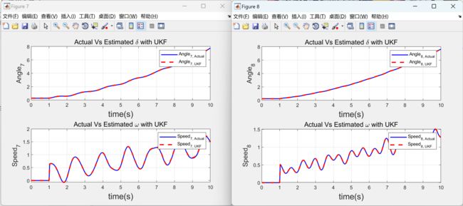
2 运行结果

2.1 UKF

 

 

 

 

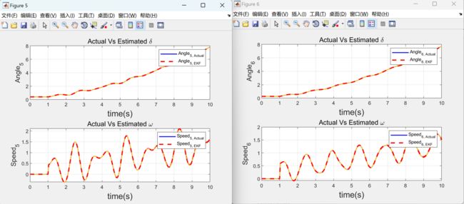
2.2 EKF 

 

 

 

 

部分代码：

% Covariance Matrix
sig=1e-2; 
P=sig^2*eye(ns);  % Error covariance matrix 
Q=sig^2*eye(ns); % system noise covariance matrix 
R=sig^2*eye(nm); % measurment noise covariance matrix 

X_hat=X_0;
X_est=[]; 
X_mes=[]; % Initial statel 

% constant values 

RMSE=[];

%Extended Kalman Filter (EKF) ALgorithm 
for k=0:deltt:t_max
    % Ybus and reconstruction matrix accodring to the requirement
    if k         ps=1;
    elseif (t_SW         ps=2;  
    else 
        ps=3; 
    end  
    
    Ybusm = YBUS(:,:,ps);
    RVm=RV(:, :, ps);
    
    [~, X] = ode45(@(t,x) dynamic_system(t,x,M,D,Ybusm,E_abs,PM,n),[k k+deltt],X_0);
    
    X_0=transpose(X(end, :));
    X_mes=[X_mes X_0];
    
    %determine the measurements 
    E1=E_abs.*exp(1j*X_0(1:n)); 
    I1=Ybusm*E1; 
    PG=real(E1.*conj(I1)); 
    QG=imag(E1.*conj(I1)); 
    Vmag=abs(RVm*E1); 
    Vangle=angle(RVm*E1); 
    z=[PG; QG; Vmag; Vangle]; 
    
    % determine Phi=df/fx 
    Phi=RK4partial(E_abs, X_hat, Ybusm, M, deltt, D, n);
    
    %prediction 
%     [~, X1]= ode45(@(t,x) dynamic_system(t,x,M,D,Ybusm,E_abs,PM,n),[k k+deltt],X_hat);
%     X_hat=transpose(X1(end, :));
    
    X_hat=RK4(n, deltt, E_abs, ns, X_hat, PM, M, D, Ybusm); 
    P=Phi*P*transpose(Phi)+Q;
    
    % correction 
    [H, zhat]=RK4H(E_abs, X_hat, Ybusm, s,n, RVm) ; 
    
    % Measurement update of state estimate and estimation error covariance 
    K=P*transpose(H)*(H*P*transpose(H)+R);
    X_hat=X_hat+K*(z-zhat); 
    P=(eye(ns)-K*H)*P; 
    
     
    X_est=[X_est, X_hat];  
    RMSE=[RMSE, sqrt(trace(P))];
end 

save('39_RMSE_EKF.mat', 'RMSE')

%% Plots
t= (0:deltt:t_max);
for i=1:1:n
figure(i)
subplot(2,1,1)
plot(t,X_mes(i, :), 'linewidth', 1.5)
hold on 
plot(t, X_est(i, :), 'linestyle', '--', 'color', 'r', 'linewidth', 2);
grid on
ylabel(sprintf('Angle_{%d}', i), 'fontsize', 12)
xlabel('time(s)', 'fontsize', 15); 
title('Actual Vs Estimated \delta', 'fontsize', 12)
legend(sprintf('Angle_{%d, Actual} ',i), sprintf('Angle_{%d, EKF}', i)); 

subplot(2,1,2)
plot(t,X_mes(i+n, :), 'linewidth', 1.5)
hold on 
plot(t, X_est(i+n, :), 'linestyle', '--', 'color', 'r', 'linewidth', 2);
grid on
ylabel(sprintf('Speed_{%d}', i), 'fontsize', 12)
xlabel('time(s)', 'fontsize', 15); 
title('Actual Vs Estimated \omega', 'fontsize', 12)
legend(sprintf('Speed_{%d, Actual} ',i), sprintf('Speed_{%d, EKF}', i));

% subplot(2,2,3)
% plot(t,X_mes(i+1, :), 'linewidth', 1.5)
% hold on 
% plot(t, X_est(i+1, :), 'linestyle', '--', 'color', 'r', 'linewidth', 2);
% grid on
% ylabel(sprintf('Angle_{%d}', i+1), 'fontsize', 12)
% xlabel('time(s)', 'fontsize', 15); 
% title('Measured Vs Eistimated \delta', 'fontsize', 12)

3 参考文献

部分理论来源于网络，如有侵权请联系删除。

4 Matlab代码实现