Braindecode系列 (2)：BCIC IV 2a 数据集上的裁剪解码

0. 引言

在Braindecode系列中，我会介绍跟BCI IV 2a有关的所有相关示例。
在Braindecode中，为训练模型创建了两种受支持的配置： trialwise decoding 和 cropped decoding。其中，trialwise decoding 已经在前面一个部分介绍了在BCIC IV 2a数据集上操作的内容，在本节中，我会接着上面的介绍第二部分的内容：BCIC IV 2a 数据集上的 cropped decoding 被用来进行更高效的数据裁剪解码。

注意：配置环境部分内容参考该系列的上一篇文章！！！

1. decoding 对比

为了更好地说明trialwise decoding 和 cropped decoding的区别，我们将通过比较来直观地解释这一点。

1.1 trialwise decoding

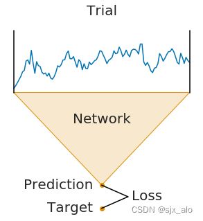
在trialwise decoding中具有以下几个特点：

1. 一个完整的Trail通过网络进行。
2. 网络产生预测。
3. 将该预测与该试验的目标（标签）进行比较，以计算损失。

1.2 cropped decoding

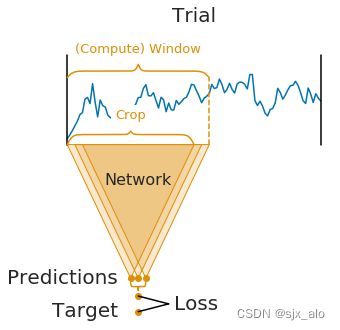
在cropped decoding中具有以下几个特点：

1. 作物不是一个完整的Trial，而是crops通过网络。
2. 为了计算效率，同时将多个相邻crops输入网络（这些相邻crops被称为计算窗口）
3. 因此，网络产生多个预测（窗口中的每个crop一个）
4. 在计算损失函数之前，对单个crop预测进行平均

1.3 两种decoding对比

• 网络架构隐含地定义了crop大小（它是感受野大小，即网络用于进行单个预测的时间步长）
• 窗口大小是一个用户定义的超参数，在Braindecode中称为“input_window_samples”。它主要影响运行时（窗口大小越大应该越快）。根据经验，您可以将其设置为crop大小的两倍。
• 裁剪大小和窗口大小一起定义了网络每个窗口进行的预测数量：window−Crop+1=predictions
• 对于cropped decoding，上述训练设置在数学上与对数据集中的Trial进行采样相同，通过网络推动它们，并直接在单个crop上进行训练。同时，上述训练设置要快得多，因为它通过使用扩张卷积避免了冗余计算。然而，只有在以下情况下，这两种设置在数学上是相同的：（1）你的网络不使用任何填充或只使用左填充（2）当使用平均输出时，你的损失函数导致相同的梯度。第一种适用于我们的浅层和深层ConvNet模型，第二种适用于PyTorch中通常用于分类的对数softmax输出和负对数似然损失。

2. Python实现

2.1 加载和预处理数据集

这部分内容同 trialwise decoding一致。具体代码如下：

from braindecode.datasets import MOABBDataset

subject_id = 3
dataset = MOABBDataset(dataset_name="BNCI2014001", subject_ids=[subject_id])

from braindecode.preprocessing import (
    exponential_moving_standardize, preprocess, Preprocessor)
from numpy import multiply

low_cut_hz = 4.  # low cut frequency for filtering
high_cut_hz = 38.  # high cut frequency for filtering
# Parameters for exponential moving standardization
factor_new = 1e-3
init_block_size = 1000
# Factor to convert from V to uV
factor = 1e6

preprocessors = [
    Preprocessor('pick_types', eeg=True, meg=False, stim=False),  # Keep EEG sensors
    Preprocessor(lambda data: multiply(data, factor)),  # Convert from V to uV
    Preprocessor('filter', l_freq=low_cut_hz, h_freq=high_cut_hz),  # Bandpass filter
    Preprocessor(exponential_moving_standardize,  # Exponential moving standardization
                 factor_new=factor_new, init_block_size=init_block_size)
]

# Transform the data
preprocess(dataset, preprocessors)

2.2 创建模型并计算窗口参数

与trialwise decoding相反，我们首先必须创建模型，然后才能将数据集剪切到窗口中。这是因为我们需要知道网络的感受野，才能知道窗口步长应该有多大。

我们首先选择将在训练期间提供给网络的计算/输入窗口大小。这必须大于网络感受野大小，否则可以选择计算效率（请参阅本教程开头的解释）。在这里，我们选择1000个样本，对于250 Hz的采样率，这是4秒。具体代码如下：

input_window_samples = 1000

随后，我们创建模型。为了使其能够有效地用于裁剪解码，我们手动将最终卷积层的长度设置为某个长度，使ConvNet的感受野小于input_window_samples（请参见模型定义中的final_conv_length=30）。具体代码如下：

import torch
from braindecode.util import set_random_seeds
from braindecode.models import ShallowFBCSPNet


cuda = torch.cuda.is_available()  # check if GPU is available, if True chooses to use it
device = 'cuda' if cuda else 'cpu'
if cuda:
    torch.backends.cudnn.benchmark = True
# Set random seed to be able to roughly reproduce results
# Note that with cudnn benchmark set to True, GPU indeterminism
# may still make results substantially different between runs.
# To obtain more consistent results at the cost of increased computation time,
# you can set `cudnn_benchmark=False` in `set_random_seeds`
# or remove `torch.backends.cudnn.benchmark = True`
seed = 20200220
set_random_seeds(seed=seed, cuda=cuda)

n_classes = 4
# Extract number of chans from dataset
n_chans = dataset[0][0].shape[0]

model = ShallowFBCSPNet(
    n_chans,
    n_classes,
    input_window_samples=input_window_samples,
    final_conv_length=30,
)

# Send model to GPU
if cuda:
    model.cuda()

随后，我们逐步将模型转换为输出密集预测的模型，这样我们就可以使用它来获得所有crops的预测。具体代码如下：

from braindecode.models import to_dense_prediction_model, get_output_shape

to_dense_prediction_model(model)

其中，为了了解模型的感受野，我们计算了虚拟输入的模型输出的形状。具体代码如下：

n_preds_per_input = get_output_shape(model, n_chans, input_window_samples)[2]

2.3 将数据剪切到窗口中

与trialwise decoding相反，我们必须为create_windows_from_events函数提供明确的窗口大小和窗口步长。具体代码如下：

from braindecode.preprocessing import create_windows_from_events

trial_start_offset_seconds = -0.5
# Extract sampling frequency, check that they are same in all datasets
sfreq = dataset.datasets[0].raw.info['sfreq']
assert all([ds.raw.info['sfreq'] == sfreq for ds in dataset.datasets])

# Calculate the trial start offset in samples.
trial_start_offset_samples = int(trial_start_offset_seconds * sfreq)

# Create windows using braindecode function for this. It needs parameters to define how
# trials should be used.
windows_dataset = create_windows_from_events(
    dataset,
    trial_start_offset_samples=trial_start_offset_samples,
    trial_stop_offset_samples=0,
    window_size_samples=input_window_samples,
    window_stride_samples=n_preds_per_input,
    drop_last_window=False,
    preload=True
)

2.4 切分数据并训练

切分数据代码同trialwise decoding，具体代码如下：

splitted = windows_dataset.split('session')
train_set = splitted['session_T']
valid_set = splitted['session_E']

在训练时，与trialwise decoding不同的是，我们现在应该向EEGClassifier提供cropped=True，并将CroppedLoss作为标准，以及criterion_loss_function作为应用于平均预测的损失函数。具体代码如下：

from skorch.callbacks import LRScheduler
from skorch.helper import predefined_split

from braindecode import EEGClassifier
from braindecode.training import CroppedLoss

# These values we found good for shallow network:
lr = 0.0625 * 0.01
weight_decay = 0

# For deep4 they should be:
# lr = 1 * 0.01
# weight_decay = 0.5 * 0.001

batch_size = 64
n_epochs = 4

clf = EEGClassifier(
    model,
    cropped=True,
    criterion=CroppedLoss,
    criterion__loss_function=torch.nn.functional.nll_loss,
    optimizer=torch.optim.AdamW,
    train_split=predefined_split(valid_set),
    optimizer__lr=lr,
    optimizer__weight_decay=weight_decay,
    iterator_train__shuffle=True,
    batch_size=batch_size,
    callbacks=[
        "accuracy", ("lr_scheduler", LRScheduler('CosineAnnealingLR', T_max=n_epochs - 1)),
    ],
    device=device,
)
# Model training for a specified number of epochs. `y` is None as it is already supplied
# in the dataset.
clf.fit(train_set, y=None, epochs=n_epochs)

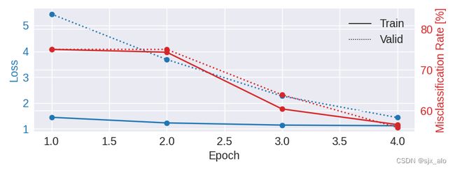
2.5 结果输出图像

最后，我们使用Skorch在整个训练过程中存储的历史来绘制精度和损失曲线。具体代码如下：

import matplotlib.pyplot as plt
from matplotlib.lines import Line2D
import pandas as pd

# Extract loss and accuracy values for plotting from history object
results_columns = ['train_loss', 'valid_loss', 'train_accuracy', 'valid_accuracy']
df = pd.DataFrame(clf.history[:, results_columns], columns=results_columns,
                  index=clf.history[:, 'epoch'])

# get percent of misclass for better visual comparison to loss
df = df.assign(train_misclass=100 - 100 * df.train_accuracy,
               valid_misclass=100 - 100 * df.valid_accuracy)

plt.style.use('seaborn')
fig, ax1 = plt.subplots(figsize=(8, 3))
df.loc[:, ['train_loss', 'valid_loss']].plot(
    ax=ax1, style=['-', ':'], marker='o', color='tab:blue', legend=False, fontsize=14)

ax1.tick_params(axis='y', labelcolor='tab:blue', labelsize=14)
ax1.set_ylabel("Loss", color='tab:blue', fontsize=14)

ax2 = ax1.twinx()  # instantiate a second axes that shares the same x-axis

df.loc[:, ['train_misclass', 'valid_misclass']].plot(
    ax=ax2, style=['-', ':'], marker='o', color='tab:red', legend=False)
ax2.tick_params(axis='y', labelcolor='tab:red', labelsize=14)
ax2.set_ylabel("Misclassification Rate [%]", color='tab:red', fontsize=14)
ax2.set_ylim(ax2.get_ylim()[0], 85)  # make some room for legend
ax1.set_xlabel("Epoch", fontsize=14)

# where some data has already been plotted to ax
handles = []
handles.append(Line2D([0], [0], color='black', linewidth=1, linestyle='-', label='Train'))
handles.append(Line2D([0], [0], color='black', linewidth=1, linestyle=':', label='Valid'))
plt.legend(handles, [h.get_label() for h in handles], fontsize=14)
plt.tight_layout()

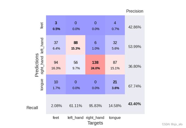
为了更好地展现结果，这里给出了绘制混淆矩阵的代码：

from sklearn.metrics import confusion_matrix
from braindecode.visualization import plot_confusion_matrix

# generate confusion matrices
# get the targets
y_true = valid_set.get_metadata().target
y_pred = clf.predict(valid_set)

# generating confusion matrix
confusion_mat = confusion_matrix(y_true, y_pred)

# add class labels
# label_dict is class_name : str -> i_class : int
label_dict = valid_set.datasets[0].windows.event_id.items()
# sort the labels by values (values are integer class labels)
labels = list(dict(sorted(list(label_dict), key=lambda kv: kv[1])).keys())

# plot the basic conf. matrix
plot_confusion_matrix(confusion_mat, class_names=labels)

3. 结果展示

这里展示了模型精度和损失变化曲线以及最后的混淆矩阵图像！！

4. 总结

到此，使用 Braindecode系列(2)：BCIC IV 2a 数据集上的裁剪解码 已经介绍完毕了！！！ 如果有什么疑问欢迎在评论区提出，对于共性问题可能会后续添加到文章介绍中。

如果觉得这篇文章对你有用，记得点赞、收藏并分享给你的小伙伴们哦。