Python-OpenCV中的图像处理

颜色空间转换

在 OpenCV 中有超过 150 中进行颜色空间转换的方法。但是你以后就会
发现我们经常用到的也就两种： BGR$Gray和BGR$HSV。

注意：在 OpenCV 的 HSV 格式中， H（色彩/色度）的取值范围是 [0， 179]，
S（饱和度）的取值范围 [0， 255]， V（亮度）的取值范围 [0， 255]。但是不
同的软件使用的值可能不同。所以当你需要拿 OpenCV 的 HSV 值与其他软
件的 HSV 值进行对比时，一定要记得归一化。

• cv2.cvtColor(img, flag)
• cv2.inRange()

import numpy as np
import cv2
from matplotlib import pyplot as plt

img1 = cv2.imread('./resource/image/opencv-logo.png', cv2.IMREAD_COLOR)
img2 = cv2.imread('./resource/image/opencv-logo.png', cv2.IMREAD_COLOR)
gray = cv2.cvtColor(img1, cv2.COLOR_BGR2GRAY)
hsv = cv2.cvtColor(img1, cv2.COLOR_BGR2HSV)
rgb = cv2.cvtColor(img1, cv2.COLOR_BGR2RGB)

imgh = np.hstack((img1, img2))
imgv = np.vstack((img1, img2)) 
cv2.imshow('hsv', hsv)
cv2.imshow('gray', gray)

plt.subplot(221), plt.imshow(imgh), plt.title('hstack')
plt.subplot(222), plt.imshow(imgv), plt.title('vstack')
plt.subplot(223), plt.imshow(hsv), plt.title('hsv')
plt.subplot(224), plt.imshow(gray), plt.title('gray')
plt.show()

物体跟踪

现在我们知道怎样将一幅图像从 BGR 转换到 HSV 了，我们可以利用这
一点来提取带有某个特定颜色的物体。在 HSV 颜色空间中要比在 BGR 空间
中更容易表示一个特定颜色。在我们的程序中，我们要提取的是一个蓝色的物
体。下面就是就是我们要做的几步：
• 从视频中获取每一帧图像
• 将图像转换到 HSV 空间
• 设置 HSV 阈值到蓝色范围。
• 获取蓝色物体，当然我们还可以做其他任何我们想做的事，比如：在蓝色
物体周围画一个圈。

import numpy as np
import cv2

# cv2.cvtColor(img, flag)
# cv2.inRange()

# 打印颜色转换flag
flags =[ i for i in dir(cv2) if i.startswith('COLOR_')]
print(flags)


# OpenCV支持超过150种颜色转换的方法，常用：BGR<->GRAY 和 BGR<->HSV
# OpenCV的HSV格式中，H(色彩/色度)的取值范围是[0, 179], S(饱和度)的取值范围[0, 255], V(亮度)的取值范围[0, 255]
# 不同软件取值范围可能不同,使用时需要做归一化

# 物体跟踪,跟踪一个蓝色物体,步骤：
# 1.从视频中获取一帧图像
# 2.将图像转换到HSV空间
# 3.设置HSV阀值到蓝色范围
# 4.获取蓝色物体,或其他处理

cap = cv2.VideoCapture(0)

while True:
    # 获取图像帧
    (ret, frame) = cap.read()

    # 转换到HSV颜色空间
    hsv = cv2.cvtColor(frame, cv2.COLOR_BGR2HSV)

    # 设定蓝色的阀值
    lower_blue = np.array([110, 50, 50])
    upper_blue = np.array([130, 255, 255])

    # 根据阀值构建掩膜
    mask = cv2.inRange(hsv, lower_blue, upper_blue)
    mask_blue = cv2.medianBlur(mask, 7)  # 中值滤波

    # 查找轮廓
    contours, hierarchy = cv2.findContours(mask_blue, cv2.RETR_EXTERNAL, cv2.CHAIN_APPROX_NONE)
    # print(contours, hierarchy)
    for cnt in contours:
        (x, y, w, h) = cv2.boundingRect(cnt)
        cv2.rectangle(frame, (x, y), (x + w, y + h), (0, 255, 0), 2)
        font = cv2.FONT_HERSHEY_SIMPLEX
        cv2.putText(frame, "Blue", (x, y - 5), font, 0.7, (0, 255, 0), 2)

    # 对原图和掩膜进行位运算
    res =cv2.bitwise_and(frame, frame, mask=mask)

    # 显示图像
    cv2.imshow('frame', frame)
    cv2.imshow('mask', mask)
    cv2.imshow('res', res)

    k = cv2.waitKey(5)&0xFF
    if k == 27:
        break

cap.release()
cv2.destroyAllWindows()

获取HSV的值

import numpy as np
import cv2

blue = np.uint8([[[255, 0, 0]]])
hsv_blue = cv2.cvtColor(blue, cv2.COLOR_BGR2HSV)
print('blue bgr:', blue)
print('blue hsv:', hsv_blue)

green = np.uint8([[[0,255,0]]])
hsv_green = cv2.cvtColor(green, cv2.COLOR_BGR2HSV)
print('green bgr:', green)
print('green hsv:', hsv_green)

red = np.uint8([[[0,0,255]]])
hsv_red = cv2.cvtColor(red, cv2.COLOR_BGR2HSV)
print('red bgr:',red)
print('red hsv:',hsv_red)

blue bgr: [[[255 0 0]]]
blue hsv: [[[120 255 255]]]
green bgr: [[[ 0 255 0]]]
green hsv: [[[ 60 255 255]]]
red bgr: [[[ 0 0 255]]]
red hsv: [[[ 0 255 255]]]

几何变换

对图像进行各种几个变换，例如移动，旋转，仿射变换等。

图像缩放

• cv2.resize()

1. cv2.INTER_AREA
2. v2.INTER_CUBIC
3. v2.INTER_LINEAR

res = cv2.resize(img, None, fx=2, fy=2, interpolation=cv2.INTER_CUBIC)
或
height, width = img.shape[:2]
res = cv2.resize(img, (2width, 2height), interpolation=cv2.INTER_CUBIC)

import numpy as np
import cv2

# 图像缩放
img = cv2.imread('./resource/image/1.jpg')

# 缩放 时推荐使用cv2.INTER_AREA 
# 扩展 时推荐使用cv2.INTER_CUBIC(慢) 或 cv2.INTER_LINEAR(默认使用)
# 原图放大两倍
res = cv2.resize(img, None, fx=2, fy=2, interpolation=cv2.INTER_CUBIC)

# 或
#height, width = img.shape[:2]
#res = cv2.resize(img, (2*width, 2*height), interpolation=cv2.INTER_CUBIC)

while True:
    cv2.imshow('res', res)
    cv2.imshow('img', img)

    if cv2.waitKey(1)&0xFF == 27:
        break
cv2.destroyAllWindows()

图像平移

OpenCV提供了使用函数cv2.warpAffine()实现图像平移效果，该函数的语法为

• cv2.warpAffine(src, M, (cols, rows))

1. src：输入的源图像
2. M：变换矩阵，即平移矩阵,M = [[1, 0, tx], [0, 1, ty]] 其中，tx和ty分别代表在x和y方向上的平移距离。
3. (cols, rows)：输出图像的大小，即变换后的图像大小

平移就是将对象换一个位置。如果你要沿（ x， y）方向移动，移动的距离
是（ tx， ty），你可以以下面的方式构建移动矩阵：
$$M=\left[\begin{array}{ccc}1& 0& t_x\\ 0& 1& t_y\end{array}\right]$$

import cv2
import numpy as np

img = cv2.imread('./resource/opencv/image/messi5.jpg')

# 获取图像的行和列
rows, cols = img.shape[:2]

# 定义平移矩阵，沿着y轴方向向下平移100个像素点
# M = np.float32([[1, 0, 0], [0, 1, 100]])

# 定义平移矩阵，沿着x轴方向向右平移50个像素点,沿着y轴方向向下平移100个像素点
M = np.float32([[1, 0, -50], [0 ,1, 100]])

# 执行平移操作
result = cv2.warpAffine(img, M, (cols, rows))

# 显示结果图像
cv2.imshow('result', result)
cv2.waitKey(0)

图像旋转

• cv2.getRotationMatrix2D()
  对一个图像旋转角度 θ, 需要使用到下面形式的旋转矩阵:
  $$M=\left[\begin{array}{cc}cos\theta & -sin\theta \\ sin\theta & cos\theta \end{array}\right]$$

import numpy as np
import cv2

# 图像旋转 缩放
img = cv2.imread('./resource/opencv/image/messi5.jpg', cv2.IMREAD_GRAYSCALE)
rows,cols = img.shape

# 这里的第一个参数为旋转中心，第二个为旋转角度，第三个为旋转后的缩放因子
# 可以通过设置旋转中心，缩放因子，以及窗口大小来防止旋转后超出边界的问题
M = cv2.getRotationMatrix2D((cols/2, rows/2), 45, 0.6)
print(M)

# 第三个参数是输出图像的尺寸中心
dst = cv2.warpAffine(img, M, (2*cols, 2*rows))
while (1):
    cv2.imshow('img', dst)
    if cv2.waitKey(1)&0xFF == 27:
        break
cv2.destroyAllWindows()

dst = cv2.warpAffine(img, M, (1cols, 1rows))

仿射变换

在仿射变换中，原图中所有的平行线在结果图像中同样平行。为了创建这
个矩阵我们需要从原图像中找到三个点以及他们在输出图像中的位置。然后
cv2.getAffineTransform 会创建一个 2x3 的矩阵，最后这个矩阵会被传给
函数 cv2.warpAffine。

import numpy as np
import cv2
from matplotlib import pyplot as plt

# 仿射变换
img = cv2.imread('./resource/opencv/image/messi5.jpg', cv2.IMREAD_COLOR)
rows, cols, ch = img.shape
img = cv2.cvtColor(img, cv2.COLOR_BGR2RGBA)

pts1 = np.float32([[50,50],[200,50],[50,200]])
pts2 = np.float32([[10,100], [200,50], [100,250]])

# 行，列，通道数
M = cv2.getAffineTransform(pts1, pts2)
dts = cv2.warpAffine(img, M, (cols, rows))

plt.subplot(121), plt.imshow(img), plt.title('Input')
plt.subplot(122), plt.imshow(dts), plt.title('Output')
plt.show()

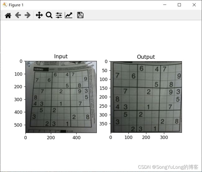
透视变换

对于视角变换，我们需要一个 3x3 变换矩阵。在变换前后直线还是直线。
要构建这个变换矩阵，你需要在输入图像上找 4 个点，以及他们在输出图
像上对应的位置。这四个点中的任意三个都不能共线。这个变换矩阵可以有
函数 cv2.getPerspectiveTransform() 构建。然后把这个矩阵传给函数
cv2.warpPerspective()

import numpy as np
import cv2
from matplotlib import pyplot as plt

# 透视变换
img = cv2.imread('./resource/opencv/image/sudoku.png', cv2.IMREAD_COLOR)
rows,cols,ch = img.shape
img = cv2.cvtColor(img, cv2.COLOR_BGR2RGB)

pts1 = np.float32([[60,80],[368,65],[28,387],[389,390]])
pts2 = np.float32([[0,0],[300,0],[0,300],[300,300]])

M = cv2.getPerspectiveTransform(pts1, pts2)
dst = cv2.warpPerspective(img, M, (400, 400))

plt.subplot(121), plt.imshow(img), plt.title('Input')
plt.subplot(122), plt.imshow(dst), plt.title('Output')
plt.show()

图像阈值

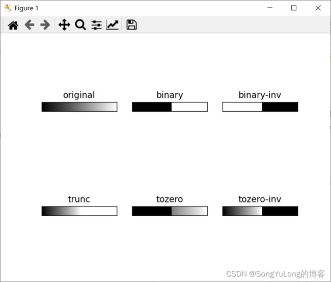
单阈值

与名字一样，这种方法非常简单。但像素值高于阈值时，我们给这个像素
赋予一个新值（可能是白色），否则我们给它赋予另外一种颜色（也许是黑色）。这个函数就是 cv2.threshhold()。这个函数的第一个参数就是原图像，原图像应该是灰度图。第二个参数就是用来对像素值进行分类的阈值。第三个参数
就是当像素值高于（有时是小于）阈值时应该被赋予的新的像素值。 OpenCV
提供了多种不同的阈值方法，这是有第四个参数来决定的。这些方法包括：

• cv2.THRESH_BINARY
• cv2.THRESH_BINARY_INV
• cv2.THRESH_TRUNC
• cv2.THRESH_TOZERO
• cv2.THRESH_TOZERO_INV

import numpy as np
import cv2
from matplotlib import pyplot as plt

# 单阈值
img = cv2.imread('./resource/opencv/image/colorscale_bone.jpg', cv2.IMREAD_GRAYSCALE)

ret,thresh1 = cv2.threshold(img, 127, 255, cv2.THRESH_BINARY)
ret,thresh2 = cv2.threshold(img, 127, 255, cv2.THRESH_BINARY_INV)
ret,thresh3 = cv2.threshold(img, 127, 255, cv2.THRESH_TRUNC)
ret,thresh4 = cv2.threshold(img, 127, 255, cv2.THRESH_TOZERO)
ret,thresh5 = cv2.threshold(img, 127, 255, cv2.THRESH_TOZERO_INV)

titles = ['original', 'binary', 'binary-inv', 'trunc', 'tozero', 'tozero-inv']
images = [img, thresh1, thresh2, thresh3, thresh4, thresh5]

for i in range(6):
    plt.subplot(2,3,i+1), plt.imshow(images[i], 'gray'),plt.title(titles[i])
    plt.xticks([]),plt.yticks([])

plt.show()

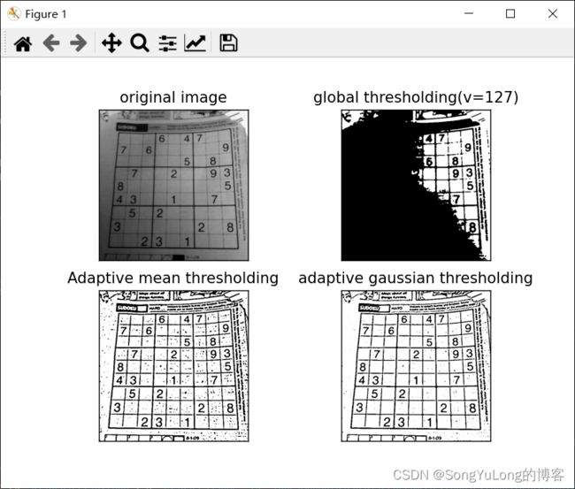
自适应阈值

在前面的部分我们使用是全局阈值，整幅图像采用同一个数作为阈值。当
时这种方法并不适应与所有情况，尤其是当同一幅图像上的不同部分的具有不
同亮度时。这种情况下我们需要采用自适应阈值。此时的阈值是根据图像上的
每一个小区域计算与其对应的阈值。因此在同一幅图像上的不同区域采用的是
不同的阈值，从而使我们能在亮度不同的情况下得到更好的结果。
这种方法需要我们指定三个参数，返回值只有一个。

• Adaptive Method- 指定计算阈值的方法。
  – cv2.ADPTIVE_THRESH_MEAN_C：阈值取自相邻区域的平
  均值
  – cv2.ADPTIVE_THRESH_GAUSSIAN_C：阈值取值相邻区域
  的加权和，权重为一个高斯窗口。
• Block Size - 邻域大小（用来计算阈值的区域大小）。
• C - 这就是是一个常数，阈值就等于的平均值或者加权平均值减去这个常
  数。

import numpy as np
import cv2
from matplotlib import pyplot as plt


# 自适应阀值
img = cv2.imread('./resource/opencv/image/sudoku.png', cv2.IMREAD_GRAYSCALE)

# 中值滤波
img = cv2.medianBlur(img, 5)

(ret, th1) = cv2.threshold(img, 127, 255, cv2.THRESH_BINARY)

# 自适应阀值 11 为block size, 2为C值
th2 = cv2.adaptiveThreshold(img, 255, cv2.ADAPTIVE_THRESH_MEAN_C, cv2.THRESH_BINARY, 11, 2)
th3 = cv2.adaptiveThreshold(img, 255, cv2.ADAPTIVE_THRESH_GAUSSIAN_C, cv2.THRESH_BINARY, 11, 2)

titles = ['original image', 'global thresholding(v=127)', 'Adaptive mean thresholding', 'adaptive gaussian thresholding']
images =[img, th1, th2, th3]


for i in range(4):
    plt.subplot(2,2,i+1), plt.imshow(images[i], 'gray')
    plt.title(titles[i])
    plt.xticks([]), plt.yticks([])

plt.show()

Otsu’s二值化

在使用全局阈值时，我们就是随便给了一个数来做阈值，那我们怎么知道
我们选取的这个数的好坏呢？答案就是不停的尝试。如果是一副双峰图像（简
单来说双峰图像是指图像直方图中存在两个峰）呢？我们岂不是应该在两个峰
之间的峰谷选一个值作为阈值？这就是 Otsu 二值化要做的。简单来说就是对
一副双峰图像自动根据其直方图计算出一个阈值。（对于非双峰图像，这种方法
得到的结果可能会不理想）。
这里用到到的函数还是 cv2.threshold()，但是需要多传入一个参数
（ flag）： cv2.THRESH_OTSU。这时要把阈值设为 0。然后算法会找到最
优阈值，这个最优阈值就是返回值 retVal。如果不使用 Otsu 二值化，返回的
retVal 值与设定的阈值相等。
下面的例子中，输入图像是一副带有噪声的图像。第一种方法，我们设
127 为全局阈值。第二种方法，我们直接使用 Otsu 二值化。第三种方法，我
们首先使用一个 5x5 的高斯核除去噪音，然后再使用 Otsu 二值化。看看噪音
去除对结果的影响有多大吧。

import numpy as np
import cv2
from matplotlib import pyplot as plt

img = cv2.imread('./resource/opencv/image/Template_Matching_Correl_Result_2.jpg', cv2.IMREAD_GRAYSCALE)

(ret1,th1) = cv2.threshold(img, 127, 255, cv2.THRESH_BINARY)
(ret2,th2) = cv2.threshold(img, 0, 255, cv2.THRESH_BINARY + cv2.THRESH_OTSU)

# (5,5)为高斯核的大小，0为标准差
blur = cv2.GaussianBlur(img, (5,5), 0) # 高斯滤波

# 阀值一定要设为0
(ret3, th3) = cv2.threshold(blur, 0, 255, cv2.THRESH_BINARY + cv2.THRESH_OTSU)

images = [img, 0, th1,
            img, 0, th2,
                img, 0, th3]
titles = ['original noisy image', 'histogram', 'global thresholding(v=127)',
            'original noisy image','histogram',"otsu's thresholding",
            'gaussian giltered image','histogram',"otus's thresholding"]

for i in range(3):
    plt.subplot(3,3,i*3+1), plt.imshow(images[i*3], 'gray')
    plt.title(titles[i*3]), plt.xticks([]), plt.yticks([])
    plt.subplot(3,3,i*3+2),plt.hist(images[i*3].ravel(),256)
    plt.title(titles[i*3+1]),plt.xticks([]),plt.yticks([])
    plt.subplot(3,3,i*3+3),plt.imshow(images[i*3+2],'gray')
    plt.title(titles[i*3+2]),plt.xticks([]),plt.yticks([])
plt.show()