使用线性回归预测票房收入 -- 机器学习项目基础篇（10）

当一部电影被制作时，导演当然希望最大化他/她的电影的收入。但是我们能通过它的类型或预算信息来预测一部电影的收入会是多少吗？这正是我们将在本文中学习的内容，我们将学习如何实现一种机器学习算法，该算法可以通过使用电影的类型和其他相关特征来预测票房收入。

数据集链接： https://drive.google.com/file/d/1D0iYGJJDUBeR8j33HUfHffEG2LJJfxIE/view

导入库和数据集

Python库使我们可以轻松地处理数据，并通过一行代码执行典型和复杂的任务。

• Pandas -此库有助于以2D数组格式加载数据框，并具有多个功能，可一次性执行分析任务。
• Numpy - Numpy数组非常快，可以在很短的时间内执行大型计算。
• Matplotlib/Seaborn -此库用于绘制可视化。
• Sklearn -该模块包含多个库，这些库具有预实现的功能，可以执行从数据预处理到模型开发和评估的任务。
• XGBoost -这包含eXtreme Gradient Boosting机器学习算法，这是帮助我们实现高精度预测的算法之一。

import numpy as np
import pandas as pd
import matplotlib.pyplot as plt
import seaborn as sb
from sklearn.model_selection import train_test_split
from sklearn.preprocessing import LabelEncoder, StandardScaler
from sklearn.feature_extraction.text import CountVectorizer
from sklearn import metrics
from xgboost import XGBRegressor
 
import warnings
warnings.filterwarnings('ignore')

现在将数据集加载到panda的数据框中。

df = pd.read_csv('boxoffice.csv',
                 encoding='latin-1')
df.head()

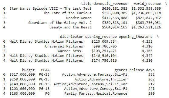
检查数据集的大小

df.shape

输出：

(2694, 10)

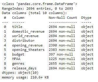
检查数据集的每列包含哪种类型的数据

df.info()

df.describe().T

数据清理

有时我们需要清理数据，因为原始数据包含大量噪声和不规则性，我们无法在这些数据上训练ML模型。因此，数据清理是任何机器学习的重要组成部分。

# We will be predicting only
# domestic_revenue in this article.
 
to_remove = ['world_revenue', 'opening_revenue']
df.drop(to_remove, axis=1, inplace=True)

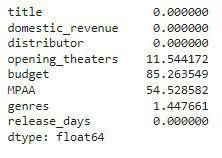
让我们检查每列中为空的条目的百分比是多少。

df.isnull().sum() * 100 / df.shape[0]

# Handling the null value columns
df.drop('budget', axis=1, inplace=True)
 
for col in ['MPAA', 'genres']:
    df[col] = df[col].fillna(df[col].mode()[0])
 
df.dropna(inplace=True)
 
df.isnull().sum().sum()

输出：

0

df['domestic_revenue'] = df['domestic_revenue'].str[1:]
 
for col in ['domestic_revenue', 'opening_theaters', 'release_days']:
    df[col] = df[col].str.replace(',', '')
 
    # Selecting rows with no null values
    # in the columns on which we are iterating.
    temp = (~df[col].isnull())
    df[temp][col] = df[temp][col].convert_dtypes(float)
 
    df[col] = pd.to_numeric(df[col], errors='coerce')

探索性数据分析（EDA）

EDA是一种使用可视化技术分析数据的方法。它用于发现趋势和模式，或在统计摘要和图形表示的帮助下检查假设。

plt.figure(figsize=(10, 5))
sb.countplot(df['MPAA'])
plt.show()

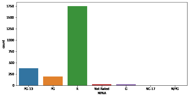
df.groupby('MPAA').mean()['domestic_revenue']

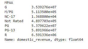
在这里，我们可以观察到PG或PG-13评级的电影通常比其他评级级别的电影收入更高。

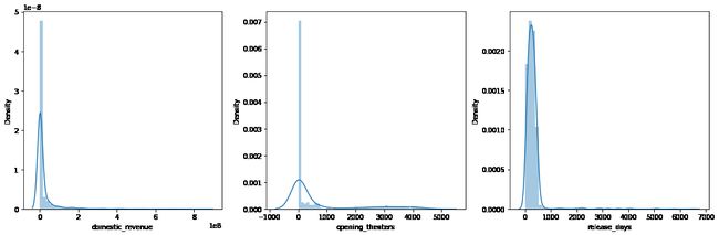
plt.subplots(figsize=(15, 5))
 
features = ['domestic_revenue', 'opening_theaters', 'release_days']
for i, col in enumerate(features):
    plt.subplot(1, 3, i+1)
    sb.distplot(df[col])
plt.tight_layout()
plt.show()

plt.subplots(figsize=(15, 5))
for i, col in enumerate(features):
    plt.subplot(1, 3, i+1)
    sb.boxplot(df[col])
plt.tight_layout()
plt.show()

当然，在上述特征中有很多离群值。

for col in features:
  df[col] = df[col].apply(lambda x: np.log10(x))

现在，我们上面可视化的列中的数据应该接近正态分布。

plt.subplots(figsize=(15, 5))
for i, col in enumerate(features):
    plt.subplot(1, 3, i+1)
    sb.distplot(df[col])
plt.tight_layout()
plt.show()

从类型创建特征

vectorizer = CountVectorizer()
vectorizer.fit(df['genres'])
features = vectorizer.transform(df['genres']).toarray()
 
genres = vectorizer.get_feature_names()
for i, name in enumerate(genres):
    df[name] = features[:, i]
 
df.drop('genres', axis=1, inplace=True)

但是会有某些类型不那么频繁，这将导致不必要地增加模型的复杂性。因此，我们将删除那些非常罕见的类型。

removed = 0
for col in df.loc[:, 'action':'western'].columns:
 
    # Removing columns having more
    # than 95% of the values as zero.
    if (df[col] == 0).mean() > 0.95:
        removed += 1
        df.drop(col, axis=1, inplace=True)
 
print(removed)
print(df.shape)

输出：

11
(2383, 24)

for col in ['distributor', 'MPAA']:
    le = LabelEncoder()
    df[col] = le.fit_transform(df[col])

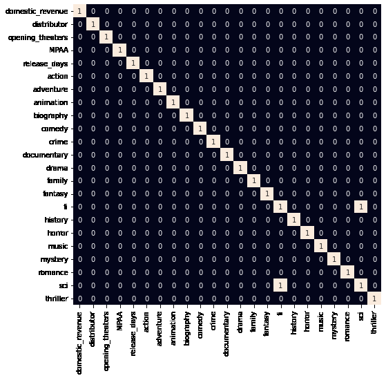
由于所有分类特征都已标记编码，让我们检查数据集中是否存在高度相关的特征。

plt.figure(figsize=(8, 8))
sb.heatmap(df.corr() > 0.8,
           annot=True,
           cbar=False)
plt.show()

模型建立

现在，我们将分离特征和目标变量，并将它们分为训练数据和测试数据，我们将使用这些数据来选择在验证数据上表现最好的模型。

features = df.drop(['title', 'domestic_revenue', 'fi'], axis=1)
target = df['domestic_revenue'].values
 
X_train, X_val,\
    Y_train, Y_val = train_test_split(features, target,
                                      test_size=0.1,
                                      random_state=22)
X_train.shape, X_val.shape

输出：

((2144, 21), (239, 21))

# Normalizing the features for stable and fast training.
scaler = StandardScaler()
X_train = scaler.fit_transform(X_train)
X_val = scaler.transform(X_val)

XGBoost库模型在大多数情况下有助于实现最先进的结果，因此，我们还将训练此模型以获得更好的结果。

from sklearn.metrics import mean_absolute_error as mae
model = XGBRegressor()
model.fit(X_train, Y_train)

我们现在可以使用剩余的验证数据集来评估模型的性能。

train_preds = models[i].predict(X_train)
print('Training Error : ', mae(Y_train, train_preds))
 
val_preds = models[i].predict(X_val)
print('Validation Error : ', mae(Y_val, val_preds))

输出：

Training Error :  0.42856612214280154
Validation Error :  0.4440195944190588

我们看到的平均绝对误差值介于预测值和实际值的对数之间，因此实际误差将高于我们上面观察到的值。