R语言实现GSEA分析（1）

传统GO和KEGG富集分析，仅可观察到多数基因富集后所在的通路，但是这些同属一条通路的基因，有的上调，有的下调，不能总体上反应这条通路是抑制还是激活。

GSEA：基因集富集分析，很好的解决了上述问题，通过观察富集的基因分布在顶端还是底部，可以说明该基因集是上调还是下降。使用R语言可以实现GSEA，具体方法R包包括：GSEABase、clusterProfiler、fgsea、gggsea。

具体操作：

1、使用clusterProfiler

#清空
rm(list=ls())
gc()
#引入包
library(clusterProfiler)
#读取差异表达数据
load("C:\\TCGA\\nrDEG_DESeq2_signif.Rdata")
alldiff<-nrDEG_DESeq2_signif[order(nrDEG_DESeq2_signif$log2FoldChange,decreasing = T),]
id <- alldiff$log2FoldChange
names(id) <- rownames(alldiff)
#读取特定基因集
immo<-clusterProfiler::read.gmt("C:\\TCGA\\c7.immunesigdb.v2023.1.Hs.symbols.gmt")
#对原始基因集进行处理
immo$term <- sub('^[^_]*_','',immo$term)#删除掉第一个下划线和之前的东西
immo.list <- immo %>% split(.$term) %>% lapply( "[[", 2)
#GSEA分析
gsea_1<-clusterProfiler::GSEA(id,TERM2GENE=immo,verbose = T)
g1<-as.data.frame(gsea_1)
g1<-subset(g1,p.adjust<0.05)
g1<-g1[order(g1$NES,decreasing = T),]
#绘图
#可视化
#绘制1个图
args(gseaplot2)
gseaplot2(gsea.re1,geneSetID = rownames(g1)[1],
          title = "",#标题
          color = "green",#颜色
          base_size = 12,#基础大小
          rel_heights = c(1.5, 0.5, 1),#小图相对高度
          subplots = 1:3,#展示小图
          pvalue_table = T,#p值表格
          ES_geom = "line"#line or dot
)
#绘制多个图
library(ggsci)
col_1<-pal_simpsons()(8)#创建了一个包含8个元素的简单色盘
num=8
gseaplot2(gsea.re1,geneSetID = rownames(g1)[1:num],
          title = "",#标题
          color = col_gsea1[1:num],#颜色
          base_size = 14,#基础大小
          rel_heights = c(1, 0.2, 0.4),#小图相对高度
          subplots = 1:3,#展示小图
          pvalue_table = F,#p值表格
          ES_geom = "line"#line or dot
)

 

 2、fgsea

library(fgsea)
immo.list_1<-immo.list[1:10]
gsea_2<-fgsea(pathways = immo.list,
              stats = id,
              minSize=1,
              maxSize=10000)
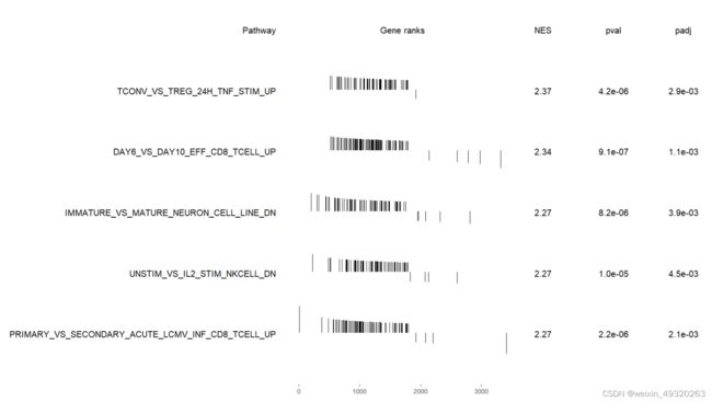
plotGseaTable(immo.list[g1$ID][1:5],
              id, 
              gsea_2,
              gseaParam = 0.5,
              colwidths = c(0.6,0.3,0.1,0.1,0.1))