【图像分类】基于LIME的CNN 图像分类研究（Matlab代码实现）

欢迎来到本博客❤️❤️

博主优势：博客内容尽量做到思维缜密，逻辑清晰，为了方便读者。

⛳️座右铭：行百里者，半于九十。

本文目录如下：

目录

1 概述

2 运行结果

3 参考文献

4 Matlab代码实现

---

1 概述

基于LIME（Local Interpretable Model-Agnostic Explanations）的CNN图像分类研究是一种用于解释CNN模型的方法。LIME是一种解释性模型，旨在提供对黑盒模型（如CNN）预测结果的可解释性。下面是简要的步骤：

1. 数据准备：首先，准备一个用于图像分类的数据集，该数据集应包含图像样本和相应的标签。可以使用已有的公开数据集，如MNIST、CIFAR-10或ImageNet。

2. 训练CNN模型：使用准备好的数据集训练一个CNN模型。可以选择常见的CNN架构，如VGG、ResNet或Inception等，或者根据具体需求设计自定义的CNN架构。

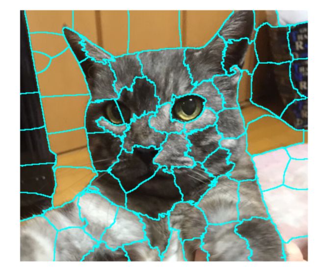
3. 解释模型的预测结果：使用LIME方法来解释CNN模型的预测结果。LIME采用局部特征解释方法，在图像中随机生成一组可解释的超像素，并对这些超像素进行采样。然后，将这些采样结果输入到CNN模型中，计算预测结果。

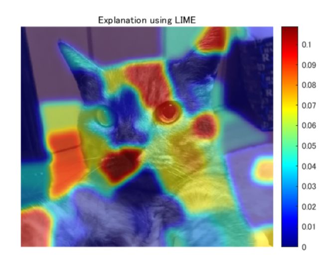
4. 生成解释性结果：根据LIME采样的结果，计算每个超像素对预测结果的影响程度。可以使用不同的解释性度量，如权重、重要性分数或热图等。

5. 分析和验证结果：对生成的解释性结果进行分析和验证。可以通过与真实标签进行对比或与其他解释方法进行比较，来评估LIME方法的准确性和可靠性。

通过以上步骤，可以实现对CNN图像分类模型的解释性研究。LIME方法可以帮助我们理解CNN模型在图像分类任务中的决策过程，对于深入了解CNN模型的特征选择和预测行为非常有帮助。

2 运行结果

result=zeros(size(L));
for i=1:N
    ROI=L==i;
    result=result+ROI.*max(mdl.Beta(i),0);% calculate the contribution if the weight is non-zero
end

% smoothing the LIME result. this is not included in the official
% implementation
result2=imgaussfilt(result,8);
% display the final result
figure;imshow(I);hold on
imagesc(result2,'AlphaData',0.5);
colormap jet;colorbar;hold off;
title("Explanation using LIME");

 部分代码：

%% Sampling for Local Exploration
% This section creates pertubated image as shown below. Each superpixel was 
% assigned 0 or 1 where the superpixel with 1 is displayed and otherwise colored 
% by black.  
% 
% 

% the number of the process to make perturbated images
% higher number of sampleNum leads to more reliable result with higher
% computation cost
sampleNum=1000;
% calculate similarity with the original image
similarity=zeros(sampleNum,1);
indices=zeros(sampleNum,N);
img=zeros(224,224,3,sampleNum);
for i=1:sampleNum
    % randomly black-out the superpixels
    ind=rand(N,1)>rand(1)*.8;
    map=zeros(size(I,1:2));
    for j=[find(ind==1)]'
        ROI=L==j;
        map=ROI+map;
    end  
    img(:,:,:,i)=imresize(I.*uint8(map),[224 224]);
    % calculate the similarity
    % other metrics for calculating similarity are also fine
    % this calculation also affetcts to the result
    similarity(i)=1-nnz(ind)./numSuperPixel;
    indices(i,:)=ind;   
end
%% Predict the perturbated images using CNN model to interpret
% Use |activations| function to explore the classification score for cat. 

prob=activations(net,uint8(img),'prob','OutputAs','rows');
score=prob(:,classIdx);
%% Fitting using weighted linear model
% Use fitrlinear function to perform weighted linear fitting. Specify the weight 
% like 'Weights',similarity. The input indices represents 1 or 0. For example, 
% if the value of the variable "indices" is [1 0 1] , the first and third superpixels 
% are active and second superpixel is masked by black. The label to predict is 
% the score with each perturbated image. Note that this similarity was calculated 
% using Kernel function in the original paper. 

sigma=.35;
weights=exp(-similarity.^2/(sigma.^2));
mdl=fitrlinear(indices,score,'Learner','leastsquares','Weights',weights);
%% 
% Confirm the exponential kernel used for the weighting. 

3 参考文献

部分理论来源于网络，如有侵权请联系删除。

[1] Ribeiro, M.T., Singh, S. and Guestrin, C., 2016, August. " Why should 
I trust you?" Explaining the predictions of any classifier. In _Proceedings 
of the 22nd ACM SIGKDD international conference on knowledge discovery and data 
mining_ (pp. 1135-1144).

[2] He, K., Zhang, X., Ren, S. and Sun, J., 2016. Deep residual learning for 
image recognition. In _Proceedings of the IEEE conference on computer vision 
and pattern recognition_ (pp. 770-778).
 

4 Matlab代码实现