逻辑斯蒂回归 - 多项式回归

一、预期结果

训练一个基于逻辑斯蒂回归的机器学习模型，它能够训练出一条二次曲线，实现二分类问题。他不是线性的，而是多项式的。

二、实验步骤

1）生成数据

首先，我们预期得到的曲线是一个二次曲线，它的方程是这样的：
y = (x - 1)**2 - 1
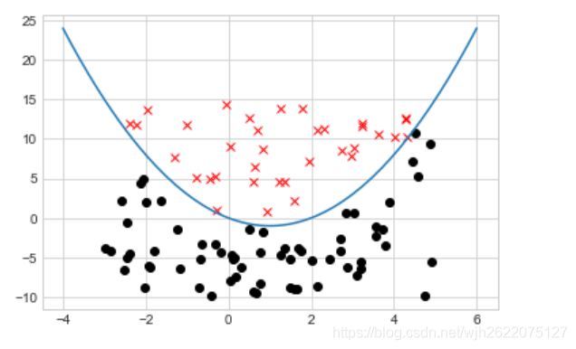
那么我们根据这个曲线生成一些数据，上下被分为两个类别
得到大概这样一张二分类图

代码实现：

import numpy as np
import random
import matplotlib.pyplot as plt
plt.style.use("seaborn-whitegrid")

# 数据有三维：（x，y，类别）
def fun(x): # 提前建立的二次曲线
    y = (x - 1)**2 - 1
    return y

def getData():
    data = []
    for i in range(100):
        x = random.uniform(-3, 5)
    #     print(x)
        y = fun(x)
        alpha = random.uniform(-5, 5)
        data.append([x, y + alpha, 0 if alpha < 0 else 1])
    data = np.array(data)
    return data

def draw(xlabel, ylabel, label):
    index0 = np.argwhere(label == 0)  # 获取值为0的数据的索引
    index1 = np.argwhere(label == 1)
    plt.plot(xlabel[index0], ylabel[index0], 'o', color='black')
    plt.plot(xlabel[index1], ylabel[index1], 'x', color='red')
    xs = np.linspace(-4, 6, 1000)
    plt.plot(xs, fun(xs))
    plt.show()

def main():
    data = getData()
    xlabel, ylabel, label = data[:, 0], data[:, 1], data[:, 2]
    draw(xlabel, ylabel, label)

if __name__ == "__main__":
    main()

想到另一种生成数据的方式，给出随机点，然后根据曲线划分类别，而不是在曲线上下生成点。

data = []
for i in range(1000):
    x = random.uniform(-3, 5)
    y = random.uniform(-10, 15)
    data.append([x, y, 0 if fun(x) > y else 1])
data = np.array(data)

这样子的似乎看上去更加自然，不像上一个凑在曲线边上了。

2）算法实现

下面就开始我们的逻辑斯谛回归算法进行回归拟合。

几个关键词：
1、sigmoid函数
2、梯度上升法

算法步骤：

1、获取规格化数据（系数矩阵、标签）

2、梯度上升法拟合系数

3、画图，看看拟合的准不准

结果

如图所示，蓝色的曲线为我们拟合到的二次曲线，而红色则为我们先前假定的曲线 在数据点不算很多的情况下，曲线也能基本拟合。

得到的方程为：y = 1.001488x^2 - 1.872946x + - 0.295519 和实际的方程y = x^2 - 2x相差不是很多。

完整代码实现：

import numpy as np
import random
import matplotlib.pyplot as plt
plt.style.use("seaborn-whitegrid")

# 数据有三维：（x，y，类别）
def fun(x): # 提前建立的二次曲线
    y = (x - 1)**2 - 1
    return y

def getData():
    data = []
    for i in range(100):
        x = random.uniform(-3, 5)
        y = random.uniform(-10, 15)
        data.append([x, y, 0 if fun(x) > y else 1])
    data = np.array(data)
    return data

def draw(xlabel, ylabel, label):
    index0 = np.argwhere(label == 0)  # 获取值为0的数据的索引
    index1 = np.argwhere(label == 1)
    plt.plot(xlabel[index0], ylabel[index0], 'o', color='black')
    plt.plot(xlabel[index1], ylabel[index1], 'x', color='red')
    xs = np.linspace(-4, 6, 1000)
    plt.plot(xs, fun(xs))
    plt.show()
    return

def sigmoid(inX):
    return 1.0 / (1 + np.exp(-inX))

def gradAscent(dataMatIn, classLabels):
    dataMatrix = np.mat(dataMatIn).transpose()
    labelMat = np.mat(classLabels).transpose()
    m, n = np.shape(dataMatrix)
    alpha = 0.0001
    maxCycles = 5000
    weights = np.ones((n, 1))
    # print(np.shape(dataMatrix)) # 100, 4
    # print(np.shape(weights)) # 4, 1
    for k in range(maxCycles):
        h = sigmoid(dataMatrix*weights)
        error = (labelMat - h) # 100, 1
        weights = weights + alpha * dataMatrix.transpose() * error
    return weights

def fun_model(weights, x):
    return (-weights[0]*x*x-weights[1]*x) / weights[2]

def drawModel(weight, xlabel, ylabel, label): # 绘制模型训练出来的图
    xs = np.linspace(-4, 6, 1000)
    index0 = np.argwhere(label == 0)  # 获取值为0的数据的索引
    index1 = np.argwhere(label == 1)
    plt.plot(xlabel[index0], ylabel[index0], 'o', color='black')
    plt.plot(xlabel[index1], ylabel[index1], 'x', color='red')
    plt.plot(xs, fun_model(weight, xs), color='blue') # 蓝色为训练出来的曲线
    plt.plot(xs, fun(xs), color='red') # 红色为假定的曲线
    plt.show()
    return

def getEquation(weight): # 根据权重得到方程
    x1 = -weight[0]/weight[2]
    x2 = -weight[1]/weight[2]
    x3 = -weight[3]/weight[2]
    equation = "y = %fx^2 %s %fx + %s %f"%(x1, '+' if x2 >= 0 else '-', abs(x2), '+' if x3 >= 0 else '-', abs(x3))
    return equation

def main():
    data = getData()
    xlabel, ylabel, label = data[:, 0], data[:, 1], data[:, 2]
    # draw(xlabel, ylabel, label) # 绘制图形
    xx = data[:, 0] ** 2
    one = np.ones(len(xx))
    new = np.array([xx, xlabel, ylabel, one])
    weights = gradAscent(new, label)
    weights = np.asarray(weights)  # np.matrix类型真的是有大坑
    # print(weights[0][0][0])
    weight = []
    for each in weights:
        weight.append(each[0])
    drawModel(weight, xlabel, ylabel, label)
    equation = getEquation(weight)
    print(equation)

if __name__ == "__main__":
    main()