基于pytorch LSTM 的股票预测

学习记录于《PyTorch深度学习项目实战100例》
https://weibaohang.blog.csdn.net/article/details/127365867?ydreferer=aHR0cHM6Ly9ibG9nLmNzZG4ubmV0L20wXzQ3MjU2MTYyL2NhdGVnb3J5XzEyMDM2MTg5Lmh0bWw%2Fc3BtPTEwMDEuMjAxNC4zMDAxLjU0ODI%3D

1.tushare

Tushare是一个免费、开源的Python财经数据接口包。主要用于提供股票及金融市场相关的数据，是国内常用的金融数据分析工具之一。Tushare对于投资研究、教学、项目背景调研等多种需求提供了极大的方便。

Tushare的主要特点有：

数据丰富：Tushare提供了包括实时行情数据、历史行情数据、基本面数据、宏观经济数据、公司基本信息、大盘指数数据、行业数据、新闻和公告等多种数据。

接口简单：使用Python调用Tushare接口相当简单。即便是初学者，只需数行代码，就能获取所需的金融数据。

社区活跃：由于Tushare的免费和开源特性，其社区相当活跃，有大量的开发者和爱好者进行维护和更新。

扩展性强：除了官方提供的数据接口，Tushare也支持自定义数据扩展，可以通过插件方式实现数据的快速扩展。

要使用Tushare，用户通常需要先进行安装，可以通过pip轻松完成。之后，通过简单的API调用，就可以获取所需的数据。

!pip install tushare

2.导入必要的依赖

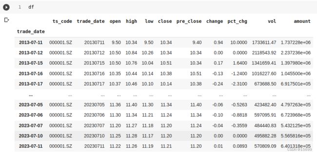
# 1.加载股票数据
pro = ts.pro_api('your-key')
df = pro.daily(ts_code='000001.SZ', start_date='20130711', end_date='20230711')

df.index = pd.to_datetime(df.trade_date)  # 索引转为日期
df = df.iloc[::-1]  # 由于获取的数据是倒序的，需要将其调整为正序

如何获取your-key

注册网站
https://tushare.pro/register

注册后进入个人主页

找到接口token

复制后粘贴 到your-key 里面

# 创建一个 StandardScaler 实例
scaler = StandardScaler()
scaler_model = StandardScaler()

# 使用 scaler 对数据进行拟合和转换
data = scaler_model.fit_transform(np.array(df[['open', 'high', 'low', 'close']]).reshape(-1, 4))

# 使用 scaler 对 'close' 列进行拟合和转换
scaler.fit_transform(np.array(df['close']).reshape(-1, 1))

分开训练集和测试集

def split_data(data,timestep):
  dataX= [] # 用于存储输入序列
  dataY= [] # 用于存储输出数据

  #将整个窗口的数据保存到X中，将未来的一天保存到Y中
  for index in range(len(data)-timestep):
    # 提取时间窗口内的数据作为输入序列
    dataX.append(data[index: index + timestep])
    # 下一个时间步的数据作为输出
    dataY.append(data[index + timestep][3]) #输出为第四列（'close' 列）

  dataX = np.array(dataX)
  dataY = np.array(dataY)

  #获取训练集大小
  train_size = int(np.round(0.8 * dataX.shape[0]))

  # 划分训练集，测试集
  x_train = dataX[: train_size, :].reshape(-1, timestep, 4)
  y_train = dataY[: train_size]

  x_test = dataX[train_size:, :].reshape(-1, timestep, 4)
  y_test = dataY[train_size:]


  return[x_train,y_train,x_test,y_test]

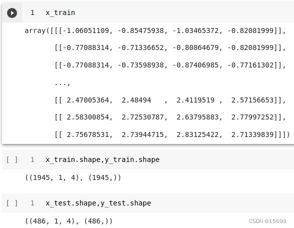
# 3.获取训练数据， x_train:1750,1,4
x_train,y_train,x_test,y_test = split_data(data,timestep=1)

探究数据集

# 4.将数据转为tensor
x_train_tensor = torch.from_numpy(x_train).to(torch.float32)
y_train_tensor = torch.from_numpy(y_train).to(torch.float32)
x_test_tensor = torch.from_numpy(x_test).to(torch.float32)
y_test_tensor = torch.from_numpy(y_test).to(torch.float32)

# 5.形成训练数据集
train_data = TensorDataset(x_train_tensor, y_train_tensor)
test_data = TensorDataset(x_test_tensor, y_test_tensor)

# 6.将数据加载成迭代器
batch_size =16
train_loader = torch.utils.data.DataLoader(train_data,
                                           batch_size,
                                           True)

test_loader = torch.utils.data.DataLoader(test_data,
                                          batch_size,
                                          False)

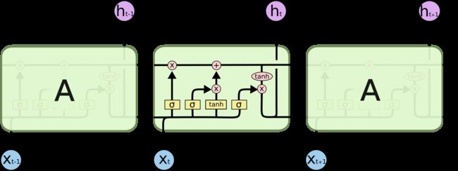
LSTM

LSTM，即长短时记忆（Long Short-Term Memory）网络，是一种特殊的循环神经网络（Recurrent Neural Network, RNN）结构。LSTM旨在解决传统RNN在处理长序列数据时容易出现的梯度消失或梯度爆炸问题。

以下是LSTM的主要组成部分和功能：

遗忘门 (Forget Gate): 决定从单元状态中删除什么信息。使用sigmoid函数，输出0表示“完全忘记”，输出1表示“完全保留”。

输入门 (Input Gate): 有两部分组成。第一部分是sigmoid层，决定哪些值我们将更新。第二部分是tanh层，创建一个新的候选值向量，它可能被加到状态中。

单元状态 (Cell State): LSTM的核心部分，其在整个链上都有运行，只有一些少量的线性交互。单元状态类似于传送带，信息可以在其上自由流动，除非受到遗忘门或输入门的影响。

输出门 (Output Gate): 决定基于单元状态输出什么值。首先，sigmoid层决定我们将输出哪些部分。然后，将单元状态通过tanh（得到值在-1到1之间）并乘以sigmoid层的输出，这样只输出我们决定的部分。

LSTM的关键优势在于其能够记住长期的依赖关系。在许多序列任务中，当前的输出不仅仅依赖于前几个步骤，还可能依赖于很早之前的步骤。LSTM相比于普通的RNN更能够捕捉这些长期依赖关系。

实际上，LSTM的变种还有很多，例如GRU（Gated Recurrent Units）。不过，无论其结构如何调整，LSTM的核心思想是利用不同的门控结构来有选择地控制信息流，从而更好地学习和记住长期依赖关系

class LSTM(nn.Module):
  def __init__(self,input_dim,hidden_dim,num_layers,output_dim):
    super(LSTM,self).__init__()
    self.hidden_dim = hidden_dim #隐藏层大小
    self.num_layers = num_layers #LSTM层数
    # input_dim 为特征维度，就是每个时间点对应的特征数量，这里为4
    self.lstm = nn.LSTM(input_dim,hidden_dim,num_layers,batch_first=True)
    self.fc = nn.Linear(hidden_dim,output_dim)

  def forward(self,x):
    # Initialize hidden state and cell state
    h0 = torch.zeros(self.num_layers, x.size(0), self.hidden_dim)
    c0 = torch.zeros(self.num_layers, x.size(0), self.hidden_dim)

    # Forward propagate through LSTM
    output, (h_n, c_n)= self.lstm(x, (h0, c0))
    batch_size, timestep, hidden_dim = output.shape

    # 将output变成 batch_size * timestep, hidden_dim
    output = output.reshape(-1, hidden_dim)
    output = self.fc(output)  # 形状为batch_size * timestep, 1
    output = output.reshape(timestep, batch_size, -1)
    return output[-1]  # 返回最后一个时间片的输出

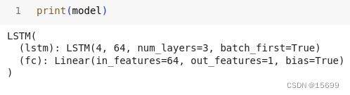
model = LSTM(input_dim, hidden_dim, num_layers, output_dim)  # 定义LSTM网络

打印模型

定义损失函数

loss_function = nn.MSELoss()  # 定义损失函数
optimizer = torch.optim.Adam(model.parameters(), lr=0.01)  # 定义优化器

配置信息

timestep = 1  # 时间步长，就是利用多少时间窗口
batch_size = 16  # 批次大小
input_dim = 4  # 每个步长对应的特征数量，就是使用每天的4个特征，最高、最低、开盘、落盘
hidden_dim = 64  # 隐层大小
output_dim = 1  # 由于是回归任务，最终输出层大小为1
num_layers = 3  # LSTM的层数
epochs = 10
best_loss = 0
model_name = 'LSTM'
save_path = './{}.pth'.format(model_name)

train

# 8. model 训练
save_path = '/content/sample_data/best.pth'
for epoch in range(epochs):
  model.train()
  running_loss= 0 #初始loss值
  train_bar = tqdm(train_loader) #通过使用tqdm来展示进度条
  for data in train_bar:
    x_train, y_train = data #
    # print(x_train.shape,y_train.shape) torch.Size([16, 1, 4]) torch.Size([16])
    optimizer.zero_grad()
    y_train_pred = model(x_train)
    loss = loss_function(y_train_pred,y_train.reshape(-1,1))
    loss.backward()
    optimizer.step()

    running_loss += loss.item()
    train_bar.desc = "train epoch[{}/{}] loss:{:.3f}".format(epoch + 1,epochs,loss) #每次你计算 loss 并更新 train_bar.desc，进度条的描述就会更新，从而实时显示你的训练 loss 和当前 epoch。
    torch.save(model.state_dict(),save_path)

加载模型

# 加载权重和偏置
model.load_state_dict(torch.load(save_path))

模型验证

# 模型验证
model.eval()
test_loss = 0
save_path_2="/content/sample_data/best_2.pth"
with torch.no_grad():
   test_bar = tqdm(test_loader)
   for data in test_bar:
      x_test, y_test = data
      y_test_pred = model(x_test)
      test_loss = loss_function(y_test_pred, y_test.reshape(-1, 1))

if test_loss < best_loss:
  best_loss = test_loss
  torch.save(model.state_dict(), save_path_2)

绘制模型

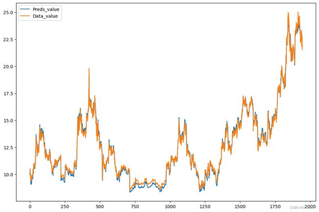
# 9.绘制结果 train 的结果
pred_value =model(x_train_tensor).detach().numpy().reshape(-1, 1)
true_value =y_train_tensor.detach().numpy().reshape(-1, 1)
plt.figure(figsize=(12, 8))
plt.plot(scaler.inverse_transform(pred_value, "b"),label="Preds_value")
plt.plot(scaler.inverse_transform(true_value, "r"),label="Data_value")
plt.legend()
plt.show()

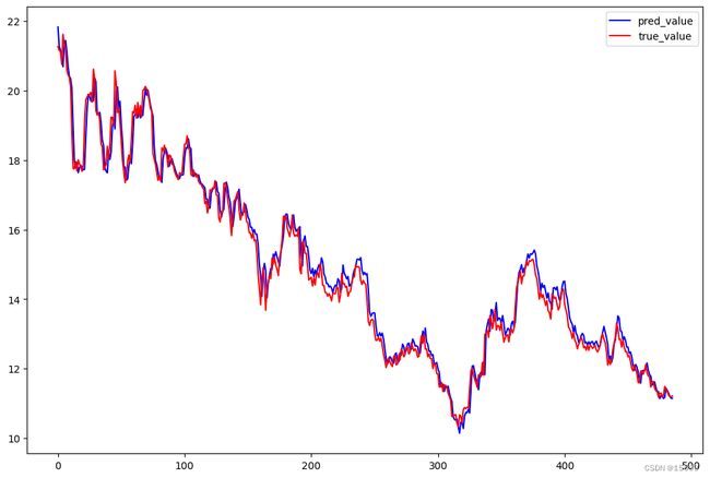
绘制test的结果

y_test_pred = model(x_test_tensor)
plt.figure(figsize=(12, 8))
plt.plot(scaler.inverse_transform(y_test_pred.detach().numpy()), "b",label="pred_value")
plt.plot(scaler.inverse_transform(y_test_tensor.detach().numpy().reshape(-1, 1)), "r",label='true_value')
plt.legend()
plt.show()

代码ipynb