FSC147数据集格式解析

一. 引言

         在研究很多深度学习框架的时候，往往需要使用到FSC147格式数据集，若要是想在自己的数据集上验证深度学习框架，就需要自己制作数据集以及相关标签，在论文Learning To Count Everything中，该数据集首次被提出。

二. FSC147数据集简介

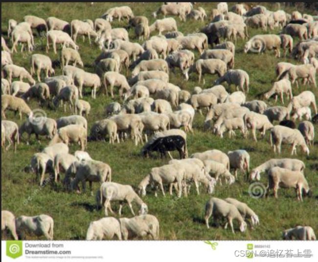
        FSC147是由147个对象类别组成的数据集，其中包含6000多张图像，适用于少镜头计数(few-shot)任务，少镜头计数大致框架可见下图。图像用两种类型标签，即点和边界框，它们可以用于开发少镜头计数模型。learning to count everything开源代码以及数据集链接：https://github.com/cvlab-stonybrook/LearningToCountEverything

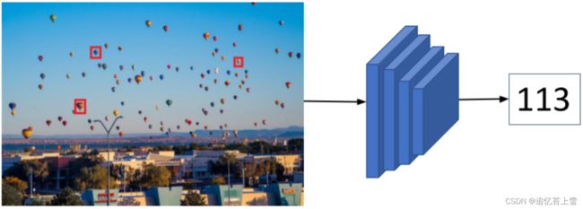
 少镜头计数(few-shot)的大致框架图

 三. FSC147数据集格式的探索

3.1 FSC147数据集的构成

        本次咱们的目标并不是探讨少镜头计数的原理以及应用，故暂且放在一边，打开FSC147数据集，我们会发现该数据集由以下几部分构成。

一个密度图文件夹，一个原图片文件夹，两个json文件，一个txt文本，下面咱们一个一个来解析

 3.2 FSC147图片类型文本

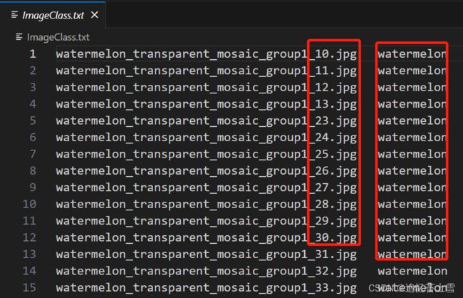
打开ImageClasses_FSC147.txt文件，发现左侧是图片的名字，右侧是图片的类型

这个比较简单，下面提供一个脚本将图片名字和目标类名传入txt文本中

其中的watermelon是图片的类名，当然，如果图片的类比较多可以自己改进一下代码，这里我只是用作测试，就没有整复杂一点

import os
import sys

path = 'D:\\Original_Images_Watermelon'   # 所需读取的文件夹路径
txt_path = 'D:\\ImageClass.txt'   # 所需写入数据的txt文档
write_txt = open(txt_path, 'w')        # 打开txt文档
for file_name in os.listdir(path):   # 读取文件夹下的文件名
    print(file_name)   # 测试一下有没有读取到信息  
    write_txt.write(file_name+'   '+'watermelon'+'\n')

输出结果如下

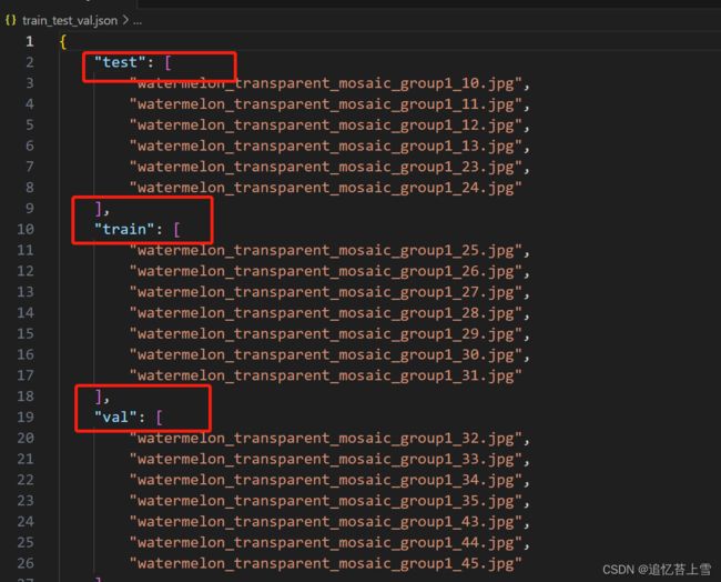
 3.3 Train_Test_Val_FSC_147.json

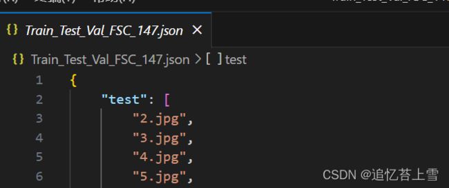
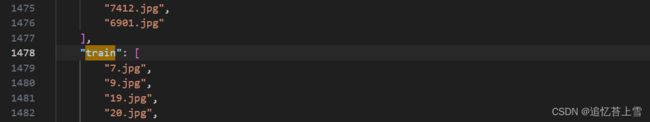
这个json文件其实很简单，打开发现就是测试集，训练集，验证集组成的图片名字的字典

 

 下面也提供一个脚本

import os
import json 
# from itertools import zip_longest    # 遍历不同长度列表的库
test_dic = {'test':[],'train':[],'val':[]}  # 创建好字典模板，其中键值对中的值是空列表用于存储所需的内容
test_name = os.listdir('D:\\Original_Images_Watermelon\\test')
train_name = os.listdir('D:\\Original_Images_Watermelon\\train')
val_name = os.listdir('D:\\Original_Images_Watermelon\\val')
# print(test_name, '\n', train_name, '\n', val_name)  # 测试有没有读取到数据
# for i, j, k in zip_longest(test_name, train_name, val_name):   这个遍历不好向字典中追加数据，因为有None元素
#     # print(i,'\n',j,'\n',k)   # 测试有没有读取到数据
#     test_dic['test'].append(i)
# print(test_dic)
# 直接采用下面简单粗暴的方式向字典中追加数据，当然，键值对太多的时候还是不建议这么干，建议研究研究上面的方法
for i in test_name:
    print(i)
    test_dic['test'].append(i)
for j in train_name:
    test_dic['train'].append(j)
for k in val_name:
    test_dic['val'].append(k)
# print(test_dic)    # 测试有没有将数据写入字典中
# 将字典内容传到json当中
with open("D:\\plant_counting\\test\\train_test_val.json", 'w') as f:
    json.dump(test_dic, f, indent=4, ensure_ascii=False)

输出结果如下，当然，我这也是小批量的验证，数据集庞大的娃可以自己改善一下代码

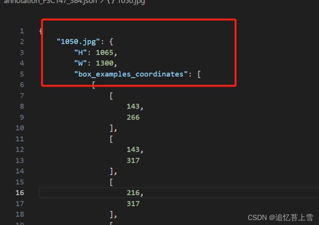
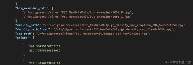
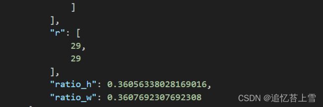
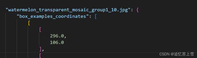
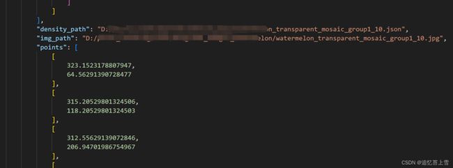
 3.4 annotation_FSC147_384.json

 这是最麻烦的一块，可以看到json文件包含了每一张图片的各种信息，其中H和W还不是原图片的尺寸，H和W乘以ratio_h和ratio_w才是原图片的尺寸，但是本人的框架用不上这个信息，在后续的脚本中我也会省去，需要的娃子可以自行根据脚本添加。

 3.4.1 fsc147的点框标签可视化

在论文中提到fsc147数据集有两种标签，一个是点一个是框

这里提供一个脚本研究一张图片，以数据集的一张图片为例子

 以下是可视化脚本，其中点和框的坐标都是从json文件中直接复制过来的

import cv2
img_path = 'D:\\plant_counting\\FSC147_384_V2\\images_384_VarV2\\1050.jpg'
img = cv2.imread(img_path)
# 以下是点坐标值
point_list =  \
[
    (
        247.53459230769232,
        212.71076056338032
    ),
    (
        247.14496153846153,
        194.39414084507044
    ),
    (
        229.89658461538463,
        66.2174647887324
    ),
    (
        251.08816923076924,
        62.02771830985916
    ),
    (
        229.66208461538463,
        51.6687323943662
    ),
    (
        254.58041538461538,
        48.35515492957747
    ),
    (
        220.28930000000003,
        78.20259154929578
    ),
    (
        156.0795923076923,
        16.762591549295777
    ),
    (
        443.8363461538462,
        342.8705352112676
    ),
    (
        452.97463076923077,
        191.4230985915493
    ),
    (
        14.358615384615383,
        38.122366197183105
    ),
    (
        30.347907692307697,
        54.88135211267606
    ),
    (
        168.57303076923077,
        121.91008450704227
    ),
    (
        48.869800000000005,
        35.0070985915493
    ),
    (
        35.2219,
        41.04653521126761
    ),
    (
        84.35145384615385,
        36.564732394366196
    ),
    (
        84.35145384615385,
        56.04957746478873
    ),
    (
        3.831369230769231,
        65.20788732394367
    ),
    (
        5.588315384615385,
        85.08214084507043
    ),
    (
        22.74289230769231,
        106.90704225352113
    ),
    (
        62.12446153846154,
        94.04574647887324
    ),
    (
        4.805446153846154,
        127.17070422535211
    ),
    (
        29.179015384615383,
        126.58659154929578
    ),
    (
        18.84297692307692,
        155.42445070422536
    ),
    (
        52.37647692307693,
        132.04191549295774
    ),
    (
        78.6982,
        128.92304225352115
    ),
    (
        100.14232307692308,
        142.17374647887326
    ),
    (
        91.17360000000001,
        113.14118309859157
    ),
    (
        103.06816153846154,
        101.84112676056338
    ),
    (
        126.46404615384617,
        120.34884507042253
    ),
    (
        103.06816153846154,
        83.1350985915493
    ),
    (
        122.36931538461539,
        41.24123943661972
    ),
    (
        130.55877692307692,
        30.33059154929578
    ),
    (
        149.07706153846155,
        39.09949295774648
    ),
    (
        9.683046153846155,
        195.367661971831
    ),
    (
        57.05565384615385,
        190.10704225352114
    ),
    (
        103.4577923076923,
        175.2987042253521
    ),
    (
        103.4577923076923,
        201.40709859154933
    ),
    (
        58.617784615384615,
        247.19864788732397
    ),
    (
        81.42561538461538,
        220.3078309859155
    ),
    (
        95.07351538461538,
        243.88507042253522
    ),
    (
        137.1861076923077,
        257.9145915492958
    ),
    (
        104.62668461538462,
        252.2645633802817
    ),
    (
        121.0056076923077,
        227.12969014084507
    ),
    (
        171.30405384615383,
        285.5842253521127
    ),
    (
        122.1745,
        156.00856338028171
    ),
    (
        152.1977153846154,
        190.30174647887324
    ),
    (
        179.4935153846154,
        183.28518309859155
    ),
    (
        162.9197769230769,
        158.73442253521128
    ),
    (
        220.62842307692307,
        180.7540281690141
    ),
    (
        258.84110000000004,
        177.24574647887323
    ),
    (
        237.7866076923077,
        156.2032676056338
    ),
    (
        213.80627692307692,
        156.59267605633804
    ),
    (
        199.5739307692308,
        152.11087323943664
    ),
    (
        11.436384615384616,
        330.398647887324
    ),
    (
        51.59721538461539,
        332.150985915493
    ),
    (
        157.0717076923077,
        340.3357746478873
    ),
    (
        203.47384615384615,
        332.150985915493
    ),
    (
        243.63467692307697,
        262.9805070422535
    ),
    (
        276.9733615384616,
        258.8881126760563
    ),
    (
        290.81607692307693,
        240.9609014084507
    ),
    (
        317.7186384615385,
        248.950985915493
    ),
    (
        312.4550153846154,
        229.85554929577467
    ),
    (
        329.2235692307692,
        312.4714366197183
    ),
    (
        352.6158461538462,
        302.5343098591549
    ),
    (
        407.4022615384616,
        240.9609014084507
    ),
    (
        418.90358461538466,
        262.9805070422535
    ),
    (
        351.44695384615386,
        237.4562253521127
    ),
    (
        426.8982307692308,
        202.38061971830984
    ),
    (
        381.66859230769234,
        181.33814084507043
    ),
    (
        343.6507307692308,
        182.89577464788732
    ),
    (
        343.6507307692308,
        167.6980281690141
    ),
    (
        329.02875384615385,
        157.95560563380283
    ),
    (
        221.99213076923078,
        125.02535211267606
    ),
    (
        207.7633923076923,
        134.3783661971831
    ),
    (
        244.99838461538462,
        138.08135211267606
    ),
    (
        268.7839,
        139.05487323943663
    ),
    (
        290.81607692307693,
        129.7018591549296
    ),
    (
        315.38085384615385,
        133.40484507042254
    ),
    (
        299.19674615384616,
        147.239661971831
    ),
    (
        249.67756153846156,
        125.41476056338028
    ),
    (
        272.09936923076924,
        156.2032676056338
    ),
    (
        225.6972307692308,
        107.68585915492959
    ),
    (
        227.45417692307694,
        93.65633802816902
    ),
    (
        153.75623846153846,
        94.43515492957748
    ),
    (
        167.9885846153846,
        81.76856338028169
    ),
    (
        176.56767692307693,
        78.45859154929578
    ),
    (
        187.87418461538462,
        68.32676056338029
    ),
    (
        411.69180769230775,
        136.13430985915494
    ),
    (
        446.7838307692308,
        149.57611267605634
    ),
    (
        445.2253076923077,
        163.80033802816902
    ),
    (
        409.1556,
        167.8927323943662
    ),
    (
        377.37904615384616,
        155.42445070422536
    ),
    (
        347.74185384615384,
        144.12078873239437
    ),
    (
        346.9625923076923,
        123.66242253521128
    ),
    (
        310.70167692307695,
        101.45171830985916
    ),
    (
        321.0341076923077,
        76.89735211267606
    ),
    (
        265.27361538461537,
        88.20101408450705
    ),
    (
        279.1163307692308,
        78.45859154929578
    ),
    (
        279.8955923076923,
        58.77904225352113
    ),
    (
        295.88488461538464,
        49.81543661971831
    ),
    (
        179.10388461538463,
        19.614647887323944
    ),
    (
        167.40413846153845,
        48.647211267605634
    ),
    (
        199.96356153846153,
        26.82230985915493
    ),
    (
        208.1530230769231,
        44.74952112676056
    ),
    (
        240.3192076923077,
        35.0070985915493
    ),
    (
        252.79821538461542,
        11.819267605633804
    ),
    (
        446.97864615384617,
        104.56698591549296
    ),
    (
        421.244976923077,
        98.72225352112677
    ),
    (
        464.52646153846155,
        91.31628169014084
    ),
    (
        458.28515384615383,
        71.44202816901408
    ),
    (
        453.6059769230769,
        65.20788732394367
    ),
    (
        421.6346076923077,
        62.08901408450704
    ),
    (
        449.70966923076924,
        57.60721126760564
    ),
    (
        391.6113923076923,
        61.50490140845071
    ),
    (
        435.08769230769235,
        42.604169014084505
    ),
    (
        459.45765384615385,
        38.710084507042254
    ),
    (
        464.3316461538462,
        33.64056338028169
    ),
    (
        442.6891,
        28.76935211267606
    ),
    (
        461.7954384615385,
        24.680563380281693
    ),
    (
        437.8151076923077,
        18.832225352112676
    ),
    (
        411.69180769230775,
        23.5087323943662
    ),
    (
        376.0117307692308,
        28.76935211267606
    ),
    (
        396.48538461538465,
        29.94118309859155
    ),
    (
        342.4782307692308,
        44.36011267605634
    ),
    (
        333.3146923076923,
        29.94118309859155
    ),
    (
        341.8937846153846,
        23.314028169014083
    ),
    (
        323.5667076923077,
        22.729915492957748
    ),
    (
        317.91345384615386,
        15.327549295774649
    ),
    (
        326.88217692307694,
        7.5321690140845075
    ),
    (
        290.0368153846154,
        18.637521126760564
    ),
    (
        297.6382230769231,
        13.961014084507042
    ),
    (
        353.98316153846156,
        11.235154929577465
    ),
    (
        361.3897538461539,
        5.9745352112676064
    ),
    (
        379.7168307692308,
        12.208676056338028
    ),
    (
        393.36473076923073,
        16.495774647887323
    )
]

for point in point_list:
    # 由于cv2.circle参数需要整形，不需要浮点型，这里要对参数做个变换
    x = int(point[0])
    y = int(point[1])
    cv2.circle(img,(x, y), 1, (255, 0, 0), -1)
cv2.rectangle(img, (143, 266), (216, 317), (0, 0, 255), 2)
cv2.rectangle(img, (297, 66), (343, 86), (0, 0, 255), 2)
cv2.rectangle(img, (151, 102), (186, 139), (0, 0, 255), 2)


save_path = '1234.jpg'
cv2.imwrite(save_path, img)

可视化效果如下，可以看到打标签的方法是所有目标都打点，选择三个目标画上框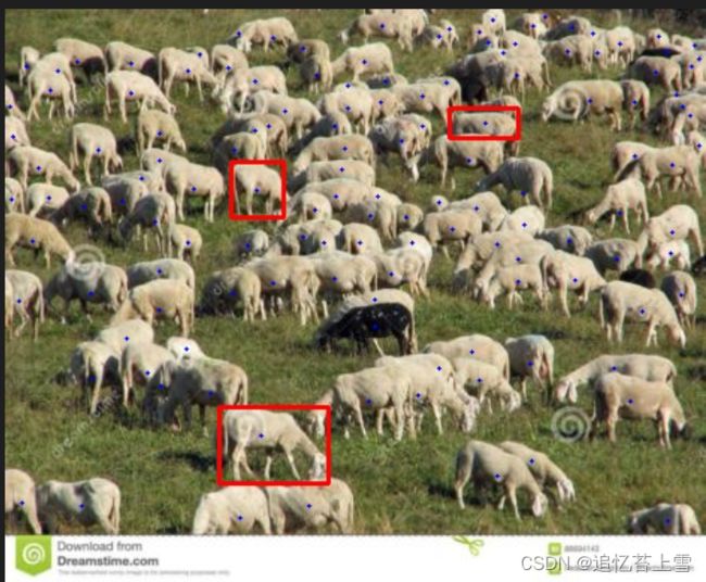

 自己利用labelme做完标签后即可按照这个上述格式进行操作

 3.4.2 密度图的制作

在fsc147数据集中，有一项是密度图，以npy为文件后缀

在本人博客中，之前介绍过密度图的生成方法，在这里附上链接：作物计数方法之合并信息生成json标签的方法_追忆苔上雪的博客-CSDN博客

 但是由于这里多了三个框标注，生成密度图需要稍微修改一下代码

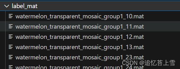
第一，要将点标签的信息提取出来并存为.mat格式的文件

import json
import numpy as np
import scipy.io as sio
import os
path = 'D:\\Label_Images_Watermelon'  # 数据集的图片路径
files = os.listdir(path)  # 返回文件夹包含名字的名字列表
for name in files:
    if name.endswith('.json'):  # 判断文件名是否以json结尾
        fp = open(os.path.join(path, name), 'r')  # 读取文件
        json_data = json.load(fp)  # 读取json格式数据
        # print(json_data)
        points_data = json_data['shapes']  # 读取shapes对象的内容
        # print(points_data, '\n')
        points = []  # 创建空列表存放每个点的位置信息
        for point in points_data:
            # print(point, '\n')   # dict_keys(['label', 'points', 'group_id', 'description', 'shape_type', 'flags'])
            if point['label'] == 'point':
                 coordinate = point['points'][0]
                 points.append(coordinate)
            else:
                print(points, type(points))
        data_inner = {'location': points, 'number': len(points)}  # 存点的位置和点的数量
        # print(data_inner, type(data_inner))  # 
        image_info = np.zeros((1,), dtype=object)
        image_info[0] = data_inner
        name = name.split('.')[0] + '.mat'
        sio.savemat(os.path.join('D:\\label_mat', name), {'image_info': image_info})

生成.mat文件如下 

 

 第二，可视化一下看看有没有问题，可视化代码如下

import json
import os, cv2
import scipy.io as io

def MatVisual1(imgpath):
    matpath = imgpath.replace('.jpg', '.mat').replace('Original_Images_Watermelon', 'label_mat')  # 图片文件对应mat文件路径
    mat = io.loadmat(matpath)  # 读取mat文件
    keypoints = mat["image_info"][0, 0][0, 0][0]  # 取出关键点坐标
    img = cv2.imread(imgpath, 1)  # 读取图片
    for keypont in keypoints:
        cv2.circle(img, (int(keypont[0]), int(keypont[1])), 1, (0, 0, 255), 4)  # 画点
    cv2.namedWindow(imgpath, 0)  # 创建窗口
    cv2.resizeWindow(imgpath, img.shape[1], img.shape[0])  # 创建窗口
    cv2.imshow(imgpath, img)
    cv2.waitKey(0)


if __name__ == "__main__":
    rootPath1 = r'./Original_Images_Watermelon'  # 图片所在路径
    imgName1 = 'watermelon_transparent_mosaic_group1_23.jpg'  # 图片名
    MatVisual1(os.path.join(rootPath1, imgName1))

可以看到提取出的信息是没有问题的

 第三，生成密度图，代码如下

import h5py
import scipy.io as io
import PIL.Image as Image
import numpy as np
import os
import glob
from matplotlib import pyplot as plt
from scipy.ndimage.filters import gaussian_filter
from scipy.spatial import KDTree
import scipy
from matplotlib import cm as cm
import warnings
warnings.filterwarnings('ignore')
def gaussian_filter_density(gt):
    print(gt.shape)
    density = np.zeros(gt.shape, dtype=np.float32)
    gt_count = np.count_nonzero(gt)
    if gt_count == 0:
        return density
    pts = np.array(list(zip(np.nonzero(gt)[1], np.nonzero(gt)[0])))
    leafsize = 2048
    # build kdtree寻找相邻目标的位置
    #  构造KDTree调用的是scipy包中封装好的函数，其中leafsize表示的是最大叶子数，如果图片中目标数量过多，可以自行修改其数值。
    tree = KDTree(pts.copy(), leafsize=leafsize)
    # query kdtree
    # tree.query（）中参数k=4查询的是与当前结点相邻三个结点的位置信息，因为distances[i][0]表示的是当前结点。
    # distances, locations = tree.query(pts, k=4)
    # 这里把源码的k = 4改成k = 3是因为目标作物的幼苗左右两侧只有两株植物
    distances, locations = tree.query(pts, k=3)
    print('generate density...')
    for i, pt in enumerate(pts):
        pt2d = np.zeros(gt.shape, dtype=np.float32)
        pt2d[pt[1], pt[0]] = 1.
        # 图像中目标比较稀疏，要重新设置高斯核
        if gt_count > 1:
            # sigma = (distances[i][1]+distances[i][2]+distances[i][3])*0.1
            sigma = (distances[i][1] + distances[i][2]) * 0.05   # 根据作物图修改的sigma
        else:
            sigma = np.average(np.array(gt.shape))/2./2.     # case: 1 point
        density += scipy.ndimage.filters.gaussian_filter(pt2d, sigma, mode='constant')
    print('done.')
    return density
if __name__ == "__main__":
    #  set the root to the dataset
    root = 'D:/plant_counting/test'
    path_sets = os.path.join(root, 'Original_Images_Watermelon')
    # print(path_sets)   # D:\苏大研究生生活\2023项目\遥感\栅格图分割\jpgImages-part
    img_paths = []
    for img_path in glob.glob(os.path.join(path_sets, '*.jpg')):
        img_paths.append(img_path)
        # print('标记', img_paths)
    # 这里为了循环保存生成的子图作为展示，以及保存生成的莫地图，将源代码的循环小小的改了一下采用enumerate()
    for p, img_path in enumerate(img_paths):
        # print(p)
        # print('1111', img_path)   # 所有文件的路径
        mat = io.loadmat(img_path.replace('.jpg', '.mat').replace('Original_Images_Watermelon', 'label_mat'))
        img= plt.imread(img_path)
        k = np.zeros((img.shape[0], img.shape[1]))
        gt = mat["image_info"][0, 0][0, 0][0]
        for i in range(0, len(gt)):
            # print(i)
            if int(gt[i][1])

 密度图如下，当然，大批量操作的时候可以不显示这个图

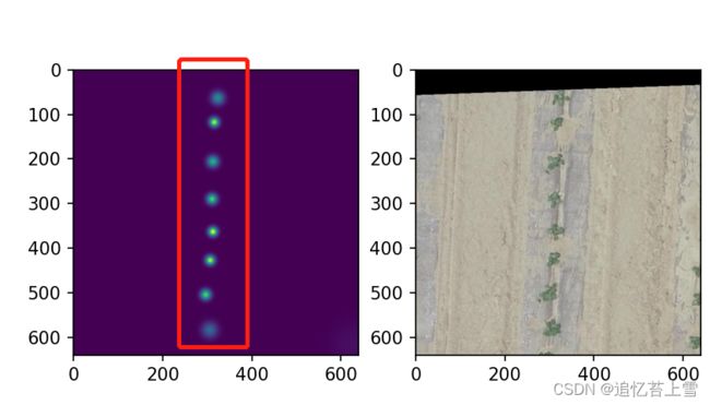
 保存的密度图如下

 

  3.4.3 annotation_FSC147_384.json制作

 前面我们把需要的信息都准备好了，就可以开始这个大的json文件制作，代码如下

import os
import json
from collections import defaultdict, OrderedDict
# 先提取外层键值对的键
path = 'D:\\Original_Images_Watermelon'
files = os.listdir(path)
# print(files)
key_outer = []   # 创建空列表储存键名
for file in files:
    file_name = os.path.basename(os.path.realpath(file))
    # print(file_name, type(file_name))     # 示例：watermelon_transparent_mosaic_group1_23.jpg
    key_outer.append(file_name)
# print(key_outer)  到这里做好了外层键名
"""获取json外层字典的内容"""
value_outer = []  # 创建空列表存储值内容
json_inner_key = {'box_examples_coordinates': '', 'density_path': '', 'img_path': '', 'points': '', }   # 先创建一个空字典
json_inner_info = ["", "", "", []]   
# 获取指定密度图路径
str_density = str('D:/density_map')
str_Img = str('D:/Original_Images_Watermelon')
label_path = 'D:\\Label_Images_Watermelon'
files = os.listdir(label_path)  # 返回文件夹包含名字的名字列表
for name in files:
    name_dir = name.split('.')[0]
    # print(name_dir)
    if name.endswith('.json'):  # 判断文件名是否以json结尾
        fp = open(os.path.join(label_path, name), 'r')  # 读取文件
        json_data = json.load(fp)  # 读取json格式数据
        # print(json_data)
        points_data = json_data['shapes']  # 读取shapes对象的内容
        # print(points_data, '\n')
        three_box_coordinate = []  # 创建空列表存储三个标注框四点的坐标
        all_points_coordinate = []  # 创建空列表存储所有标注点的坐标
        for point in points_data:
            left_bottom = []
            right_up = []  # 创建空列表存储框标签左下角和右上角的坐标
            box_coordinate = []   # 创建空列存储标注框四点的坐标
            # print(point, point.keys())  # dict_keys(['label', 'points', 'group_id', 'description', 'shape_type', 'flags'])
            if point['label'] == 'point':
                # print(point['points'][0])    # point['points'][0]就是每个点(点标注)的坐标,如[302.7354260089686, 30.53811659192826]
                coordinate = point['points'][0]  # -----------提取点标注坐标值---------------
                all_points_coordinate.append(coordinate)  # --------------------所有标注点点坐标-------------
            elif point['label'] == 'box':
                left_up = point['points'][0]   # 框标注左上角的坐标
                right_bottom = point['points'][1]  # 框标注右下角的坐标
                left_bottom.append(left_up[0])
                left_bottom.append(right_bottom[1])    # 框标注左下角坐标
                right_up.append(right_bottom[0])
                right_up.append(left_up[1])            # 框标注右上角坐标值
                box_coordinate.append(left_up)
                box_coordinate.append(left_bottom)
                box_coordinate.append(right_bottom)
                box_coordinate.append(right_up)     
                three_box_coordinate.append(box_coordinate)      # --------------------三个标注框各点坐标-------------
            print(all_points_coordinate, '\n')
            print(three_box_coordinate, '\n')
        density_path_dir = str_density + '/' + name_dir + '.json'     # --------------------密度图路径--------------
        Img_path_dir = str_Img + '/' + name_dir + '.jpg'
        json_inner_info[0] = three_box_coordinate  # 指定更新列表的数值
        # print(json_inner_info, '\n')
        json_inner_info[1] = density_path_dir  # 指定更新列表的数值
        json_inner_info[2] = Img_path_dir
        json_inner_info[3] = all_points_coordinate
        json_inner = dict(zip(json_inner_key.keys(), json_inner_info))
        value_outer.append(json_inner)
        print(value_outer, '\n')
json_fin = dict(zip(key_outer, value_outer))   # 键值对匹配成新的字典
# print(json_fin)
# 将字典传入json文件中，字典内容写入json时，需要用json.dumps将字典转换为字符串，然后再写入
with open('annotation_watermelon.json', 'w', encoding='utf-8') as f:
    json.dump(json_fin, f, indent=4, sort_keys=True, ensure_ascii=False)
    # 使用indent=4 参数来对json进行数据格式化输出，会根据数据格式缩进显示，读起来更加清晰
    # Key是文本的时候，如果sort_keys是False，则随机打印结果，如果sortkeys为true，则按顺序打印, 这里要顺序写入
    # json在进行序列化时，默认使用的是编码是ASCII，而中文为Unicode编码，ASCII中不包含中文，所以出现了乱码。
    # 想要json.dumps()能正常显示中文，只要加入参数ensure_ascii=False即可，这样json在序列化的时候，就不会使用默认的ASCII编码
# # 读取annotation_watermelon.json看看效果
# with open('annotation_watermelon.json', encoding='utf-8') as f:
#     json_file = json.load(f)
# print(json_file)    # 打印一下生成的json文件看看有没有问题

 最终生成的json大标签如下

 到这里我们的工作就完成了

 四. 声明

1. 以上提供的代码，路径我都去掉了一部分隐私信息，大家自己做的时候需要根据自己的文件路径调整

2. 路径中最好不要出现中文；

3. 本文未经本人同意不得转载或者盗用；

4. 喜欢本文请多多点赞收藏，谢谢。