李宏毅-21-hw3:对11种食物进行分类-CNN

一、代码慢慢阅读理解+总结内化：

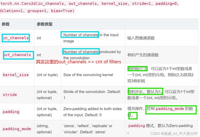
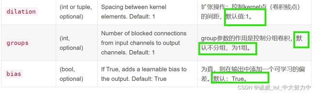
1.关于torch.nn.covd2d()的参数含义、具体用法、功能：

（1）参数含义：

注意，里面的“padding”参数：《both》side所以是上下左右《四》边都会加一个padding数量的0列:

证明如下：

import torch

x = torch.randn(3,1,5,4)
print(x)

conv = torch.nn.Conv2d(1,4,3,1,1)
res = conv(x)

print(res.shape)    # torch.Size([3, 4, 5, 4])
#所以说，很明显，只要padding的参数设置为1 + filter大小为3*3，那么输出的图像高、宽==输入的高、宽

运行结果：torch.Size([3, 4, 5, 4]

(2)具体用法：

import torch

x = torch.randn(3,1,5,4)
print(x)

conv = torch.nn.Conv2d(1,4,(2,3))
res = conv(x)

print(res.shape)    # torch.Size([3, 4, 4, 2])

输入：x[ batch_size, channels, height_1, width_1 ]
batch_size，一个batch中样本的个数 3
channels，通道数，也就是当前层的深度 1
height_1， 图片的高 5
width_1， 图片的宽 4

卷积操作：Conv2d[ channels, output, height_2, width_2 ]
channels，通道数，和上面保持一致，也就是当前层的深度 1
output ，输出的深度 4【需要4个filter】
height_2，卷积核的高 2
width_2，卷积核的宽 3

输出：res[ batch_size,output, height_3, width_3 ]
batch_size,，一个batch中样例的个数，同上 3
output， 输出的深度 4
height_3， 卷积结果的高度 4
width_3，卷积结果的宽度 2

（3）功能：

里面实现的功能,应该就是实现利用自己设定数量的filters，进行按照自己设定的stride、padding的方式对整个图像进行二维卷积，得到一个新的channel的图像,

新的channels的数目 == filters的数目,

至于输出的图像的size，需要自己进行计算一下！！！

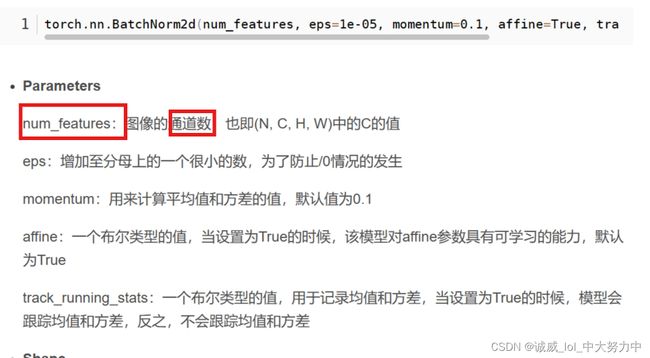
2.torch.nn.BatchNorm2d()的参数含义、用法、功能作用：

（1）参数含义:

（2）用法示例：

里面看到的randn()

输入：x[ batch_size, channels, height_1, width_1 ]
batch_size，一个batch中样本的个数 2，也就是有2个tensor张量，后面3是张量的厚、高、宽

channel的大小是3

高、宽都是2

import torch.nn as nn
import torch
if __name__ == '__main__':
    bn = nn.BatchNorm2d(3)
    ip = torch.randn(2, 3, 2, 2)
    print(ip)
    output = bn(ip)
    print(output)

（3）功能作用：

BatchNorm为什么NB呢，关键还是效果好。①不仅仅极大提升了训练速度，收敛过程大大加快；②还能增加分类效果，一种解释是这是类似于Dropout的一种防止过拟合的正则化表达方式，所以不用Dropout也能达到相当的效果；③另外调参过程也简单多了，对于初始化要求没那么高，而且可以使用大的学习率等。总而言之，经过这么简单的变换，带来的好处多得很，这也是为何现在BN这么快流行起来的原因。

具体参见这一篇文章：白话详细解读（七）----- Batch Normalization_底层研究生的博客-CSDN博客

3.torch.nn.MaxPool2d()最大池化（pooling）函数：

(1)参数含义：

nn.MaxPool2d(2, 2, 0), #但是pooling会改变图像的大小,图像会变成64*（128/2）*(128/2)

第一个“2”： 代表kernel_size,也就是窗口的大小，这里只有1个数值，那就是正方形的了

第二个“2”：代表stride，这里只有1个数值，那么就是向右的时候2个，向下的时候，也是2个

第三个“0”：代表在4个边加padding层的层数

（2）用法示例：

torch.nn.MaxPool2d详解_Medlen的博客-CSDN博客

具体可以参见这一篇博客，每个参数的用法讲述得非常详细

（3）作用：

主要是为了减少图像的高、宽size，和图像压缩的思想一致，也是利用了对于“下采样”的话，人眼对图像的感知是不会发生改变的

4.DataLoader的使用-初探：

（1）一个最基础的实例：

import torch
from torch.utils.data import Dataset, DataLoader
#下面逐步分析如下创建Dataset 和 DataLoader的示例代码

#1.从已经定义好的Dataset基类中继承得到Plus1Dataset类
class Plus1Dataset(Dataset):
     def __init__(self, a=0, b=1): #（1）定义这个类的构造函数，self是固定的要求，a,b是自己设置的变量
         super(Dataset, self).__init__()#继承得到积累的构造函数
         assert a <= b #需要a<=b,否则终断开(断言语法)
         self.a = a
         self.b = b
        
     def __len__(self):
         return self.b - self.a + 1 #（2）定义len函数，返回b-a+1
        
     def __getitem__(self, index): #（3）定义getitem函数，有一个参数index,一般都是返回这个index位置的那一行数据
        assert self.a-1 <= index <= self.b-1
        return index, index+1
#2.实例化创建Plus1Dataset和DataLoader的对象
data_train = Plus1Dataset(a=1,b=16)
data_train_loader = DataLoader(data_train, batch_size=4, shuffle=True)
print(len(data_train))  

从这个实例可以看出，

Dataset只是一个数据的容器，它是Loader的一部分

但是呢，DataLoader里面不仅有数据，还有对数据进行处理的方法，比如batch_size的大小，是否shuffle等

(2)http://t.csdn.cn/6H0LG

这个文章里面讲述得还算比较清晰，不过需要下载CIFAR-10的数据集

5.利用matplotlib中的plt.imread读取(同一个文件夹下)，plt.imshow和plt.show打印输出图像

import matplotlib.pyplot as plt

test = plt.imread("./00000000.png")

plt.imshow(test)
plt.axis('off')  # 关闭坐标轴
plt.show()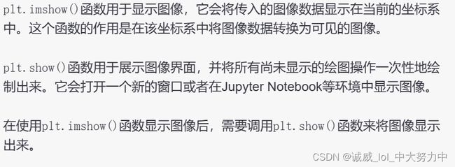

6.使用PIL库中的Image进行操作图像：

from PIL import Image

# Load the image
image = Image.open("image.jpg")

# Save the image with a new name and format
output_path = "output.png"
image.save(output_path, "PNG")

# Show the output path
print("Image saved at:", output_path)

通过Image.open打开的对象可以直接作为transforms的参数，它可以和numpy.array进行转换，上面用plt打开的方式其实得到的是numpy.array对象，不能直接transform

7.torchvision.transforms模块-初探：

慢慢阅读学习+自己实践一下是否可以对一个图像进行这样的处理

import matplotlib.pyplot as plt
from PIL import Image
test = plt.imread("./00000000.png")
test2 = Image.open("00000000.png")

#plt.imshow(test)
#plt.axis('off')

#plt.show()
mean = [0.485, 0.456, 0.406]
std = [0.229, 0.224, 0.225]



import torchvision.transforms as transforms
train_transforms =transforms.Compose([
    transforms.Resize((500,500)), #这个函数可以将图像转变为统一的500*500的大小
    #transforms.CenterCrop(300), #这个就是从中心裁剪300*300的大小的图片，原来其他部分都不要了
    #transforms.RandomCrop(300), #随机裁剪出一个300*300部分
    #transforms.RandomHorizontalFlip(0.5),#以0.5个概率进行水平翻转
    #transforms.RandomRotation(degrees=45),#在不超过45度的范围内进行随机旋转
    #transforms.Normalize(mean = mean,std=std) #反正就是 归一化，没什么好说的
    #transforms.ToTensor(),#这个用得挺多的，就是将图像转换为tensor的数据类型
    #transforms.ColorJitter(brightness=0.5,contrast=0.5,saturation=0.5,hue=0.5),#分别设置亮度，对比度，饱和度，色调的偏差范围[随机]
    #transforms.Grayscale(), #将图像转变为channel==1的灰度图
    
    
])

img1 = train_transforms(test2)

#下面是存储一个Image类型的图片放到该目录下的方式
save_path = "test_output.png"
img1.save(save_path,"PNG")
print("Image as below:",save_path)

img1.show() #似乎Image只有这个函数可以显示图像，而且是用默认图像查看器打开的，算了，就这样吧
#和上面的plt有些不同plt是在下面输出显示绘制

8.torch.nn.Softmax()函数讲解：

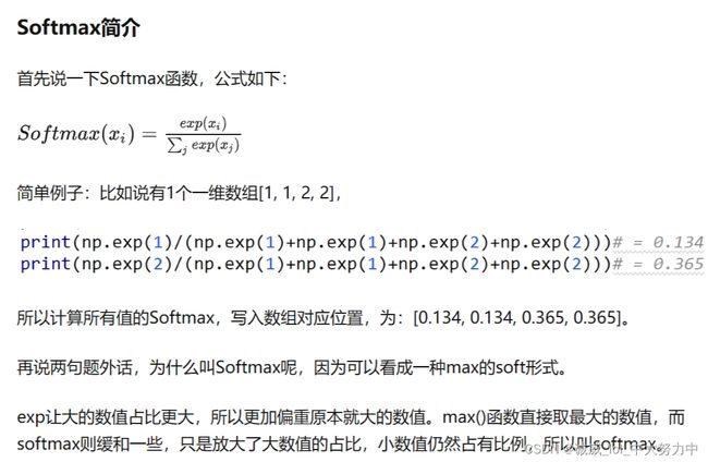
Pytorch nn.Softmax(dim=?) - 知乎 (zhihu.com)

这篇文章中详细讲解了 Softmax函数中的dim参数的用法：

这篇文章描述得非常清晰，比chatGPT讲的好多了

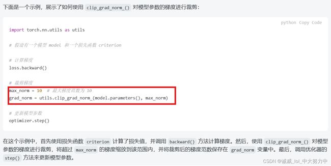
9.防止梯度爆炸的函数utils.clip_grad_norm(,)的用法：

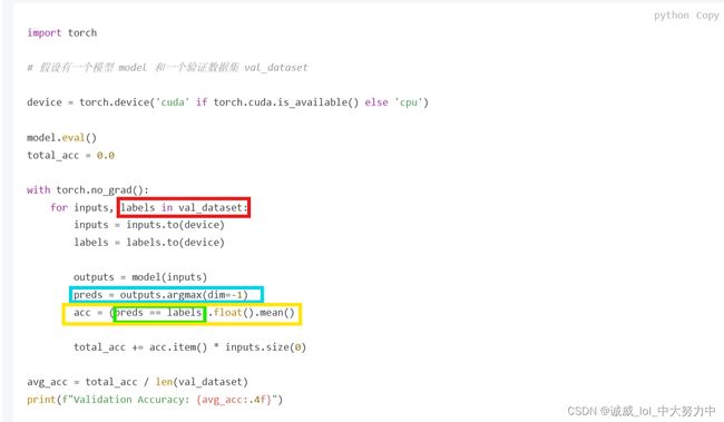
10.调用argmax函数，在最后一个维度中的每一组的抽取出max值的位置索引组成一个向量，用于和label中的数据进行比较，从而计算accuracy：

二、定义的基本classifier模型：

class Classifier(nn.Module): #这里定义了这个CNN食物图像分类的nuaral network结构
    def __init__(self):
        super(Classifier, self).__init__()
        # The arguments for commonly used modules:
        # torch.nn.Conv2d(in_channels, out_channels, kernel_size, stride, padding)
        # torch.nn.MaxPool2d(kernel_size, stride, padding)

        # input image size: [3, 128, 128]
        #需要我进一步进行慢慢学习的是：
        #（1）这个Convd函数的参数的意义？以及具体的实现是什么？
        #答：里面实现的功能,应该就是实现利用自己设定数量的filters，进行按照自己设定的stride、padding的方式对整个图像进行二维卷积，得到一个新的channel的图像
        #...具体见csdn
        #（2）这个BatchNorm2d函数的参数的意义？以及实现的功能是什么
        #（3）这里特别需要注意的是，这次用的数据是图像，最开始有对图像进行transform.resize(128,128),所以图像的pixel大小应该是3*128*128
        #所以，这个图像数据到底经历了什么？
        self.cnn_layers = nn.Sequential(
            nn.Conv2d(3, 64, 3, 1, 1), #通过我的计算，输出的大小应该是64[厚]*128[高]*128[宽]
            nn.BatchNorm2d(64), #参数是channels（filters）的数量，只会改变数据分布，不会改变数据形状
            nn.ReLU(), #先通过BN,再使用ReLU是真的香，这样就可以最大化的利用BN得到的（0，1）正太分布了
            nn.MaxPool2d(2, 2, 0),#但是pooling会改变图像的大小,图像会变成64*（128/2）*(128/2)

            nn.Conv2d(64, 128, 3, 1, 1),
            nn.BatchNorm2d(128),
            nn.ReLU(),
            nn.MaxPool2d(2, 2, 0),#图像大小128*32*32

            nn.Conv2d(128, 256, 3, 1, 1),
            nn.BatchNorm2d(256),
            nn.ReLU(),
            nn.MaxPool2d(4, 4, 0),#图像大小256*8*8
        )
        self.fc_layers = nn.Sequential(
            nn.Linear(256 * 8 * 8, 256),
            nn.ReLU(),
            nn.Linear(256, 256),
            nn.ReLU(),
            nn.Linear(256, 11)
        )

    def forward(self, x):
        # input (x): [batch_size, 3, 128, 128]
        # output: [batch_size, 11]

        # Extract features by convolutional layers.
        x = self.cnn_layers(x)

        # The extracted feature map must be flatten before going to fully-connected layers.
        x = x.flatten(1) #需要展平之后，才能调用Linear()层

        # The features are transformed by fully-connected layers to obtain the final logits.
        x = self.fc_layers(x)
        return x

三、定义get_pseudo_labels函数:

这个函数，就是为了使用哪些没有label的数据，从而实现semi-unsupervised的训练方式，这里暂时先不考虑

def get_pseudo_labels(dataset, model, threshold=0.65): #参数是dataset,model和门槛
    # This functions generates pseudo-labels of a dataset using given model.
    # It returns an instance of DatasetFolder containing images whose prediction confidences exceed a given threshold.
    # You are NOT allowed to use any models trained on external data for pseudo-labeling.
    device = "cuda" if torch.cuda.is_available() else "cpu"#设备选择

    # Construct a data loader.
    data_loader = DataLoader(dataset, batch_size=batch_size, shuffle=False) #创建一个data_loader

    # Make sure the model is in eval mode.
    model.eval()
    # Define softmax function.
    softmax = nn.Softmax(dim=-1)

    # Iterate over the dataset by batches.
    for batch in tqdm(data_loader):
        img, _ = batch

        # Forward the data
        # Using torch.no_grad() accelerates the forward process.
        with torch.no_grad():
            logits = model(img.to(device))

        # Obtain the probability distributions by applying softmax on logits.
        probs = softmax(logits)

        # ---------- TODO ----------
        # Filter the data and construct a new dataset.

    # # Turn off the eval mode.
    model.train()
    return dataset

四、train部分：

# ---------- Training ----------
    # Make sure the model is in train mode before training.
    model.train() #开启train模式

    # These are used to record information in training.
    train_loss = [] #准备好记录train过程中的loss数值和accuracy的数值
    train_accs = []

    # Iterate the training set by batches.
    for batch in tqdm(train_loader): #每一个batch中进行的操作

        # A batch consists of image data and corresponding labels.
        imgs, labels = batch #从这个batch中获取到imgs数据数组 和 labels数据数组

        # Forward the data. (Make sure data and model are on the same device.)
        logits = model(imgs.to(device)) #计算出这一个batch的logits

        # Calculate the cross-entropy loss.
        # We don't need to apply softmax before computing cross-entropy as it is done automatically.
        loss = criterion(logits, labels.to(device)) #计算logits和labels之间的loss

        # Gradients stored in the parameters in the previous step should be cleared out first.
        optimizer.zero_grad() #清空之前的grad

        # Compute the gradients for parameters.
        loss.backward()

        # Clip the gradient norms for stable training.
        grad_norm = nn.utils.clip_grad_norm_(model.parameters(), max_norm=10)

        # Update the parameters with computed gradients.
        optimizer.step() #调用backward+step进行常规化的模型更新 + clip_grad_norm防止梯度爆炸

        # Compute the accuracy for current batch.
        acc = (logits.argmax(dim=-1) == labels.to(device)).float().mean()

        # Record the loss and accuracy.
        train_loss.append(loss.item()) #将这个batch的loss放到数组中
        train_accs.append(acc)     #将这个batch的acc放到数组中
    #一个epoch完成，接下来就是计算这一次的均值，然后进行打印输出
    # The average loss and accuracy of the training set is the average of the recorded values.
    train_loss = sum(train_loss) / len(train_loss) 
    train_acc = sum(train_accs) / len(train_accs)

    # Print the information.
    print(f"[ Train | {epoch + 1:03d}/{n_epochs:03d} ] loss = {train_loss:.5f}, acc = {train_acc:.5f}")

五、validation部分：

 #validtion部分和train部分基本一样，处理backward+step哪里不需要了
    # ---------- Validation ----------
    # Make sure the model is in eval mode so that some modules like dropout are disabled and work normally.
    model.eval()

    # These are used to record information in validation.
    valid_loss = []
    valid_accs = []

    # Iterate the validation set by batches.
    for batch in tqdm(valid_loader):

        # A batch consists of image data and corresponding labels.
        imgs, labels = batch

        # We don't need gradient in validation.
        # Using torch.no_grad() accelerates the forward process.
        with torch.no_grad():
          logits = model(imgs.to(device))

        # We can still compute the loss (but not the gradient).
        loss = criterion(logits, labels.to(device))

        # Compute the accuracy for current batch.
        acc = (logits.argmax(dim=-1) == labels.to(device)).float().mean()

        # Record the loss and accuracy.
        valid_loss.append(loss.item())
        valid_accs.append(acc)

    # The average loss and accuracy for entire validation set is the average of the recorded values.
    valid_loss = sum(valid_loss) / len(valid_loss)
    valid_acc = sum(valid_accs) / len(valid_accs)

    # Print the information.
    print(f"[ Valid | {epoch + 1:03d}/{n_epochs:03d} ] loss = {valid_loss:.5f}, acc = {valid_acc:.5f}")

六、test部分：

# Make sure the model is in eval mode.
# Some modules like Dropout or BatchNorm affect if the model is in training mode.
model.eval()

# Initialize a list to store the predictions.
predictions = [] #开启eval()模式后，设置一个pred数组，用于存储通过model计算得到的预测结果，之后用于和labels进行比较

# Iterate the testing set by batches.
for batch in tqdm(test_loader): #还是利用tqdm进行迭代,一个个的batch进行处理
    # A batch consists of image data and corresponding labels.
    # But here the variable "labels" is useless since we do not have the ground-truth.
    # If printing out the labels, you will find that it is always 0.
    # This is because the wrapper (DatasetFolder) returns images and labels for each batch,
    # so we have to create fake labels to make it work normally.
    imgs, labels = batch #获取图像数据

    # We don't need gradient in testing, and we don't even have labels to compute loss.
    # Using torch.no_grad() accelerates the forward process.
    with torch.no_grad():
        logits = model(imgs.to(device)) #计算得到预测的结果

    # Take the class with greatest logit as prediction and record it.
    predictions.extend(logits.argmax(dim=-1).cpu().numpy().tolist()) #直接将预测的logits转换为preditions里面一些one-hot vec

七、创建predict.csv文件，并且将prediction数组中的结果进行写入:

# Save predictions into the file.
with open("predict.csv", "w") as f: #创建一个predict.csv文件

    # The first row must be "Id, Category"
    f.write("Id,Category\n")  #第一行是:Id, Category

    # For the rest of the rows, each image id corresponds to a predicted class.
    for i, pred in  enumerate(predictions): #将predictions中的结果逐个写入到这个文件中
         f.write(f"{i},{pred}\n")

训练的结果，就算是sample的代码用T4,也要跑25分钟才能跑完80个epoch

(1)这是用sample代码跑34个epoch时的 accuracy，在train上面已经很好了，但是在valid上面还是处于50%左右

(2)在第40个epoch时，出现了突破：

之后的结果就之后再说。。。