【重新定义matlab强大系列十四】基于问题求解有/无约束非线性优化

 运行环境：Matlab

 撰写作者：左手の明天

 精选专栏：《python》

  推荐专栏：《算法研究》

#### 防伪水印——左手の明天 ####

大家好，我是左手の明天！好久不见

今天开启新的系列——重新定义matlab强大系列

  最近更新：2023 年 09 月 23 日，左手の明天的第 291 篇原创博客

 更新于专栏：matlab

#### 防伪水印——左手の明天 ####

---

约束优化定义

约束最小化问题求向量 x，在满足 x 取值约束的前提下，使得标量函数 f(x) 取得局部最小值：

使得以下一项或多项成立：c(x) ≤ 0, ceq(x) = 0, A·x ≤ b, Aeq·x = beq, l ≤ x ≤ u。 

基于问题求解非线性优化

通过使用基于问题的方法寻找具有非线性约束的非线性目标函数的最小值。要使用基于问题的方法找到非线性目标函数的最小值，首先将目标函数编写为文件或匿名函数。目标函数是

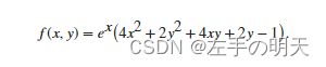
type objfunx


function f = objfunx(x,y)
f = exp(x).*(4*x.^2 + 2*y.^2 + 4*x.*y + 2*y - 1);
end

创建优化问题变量 x 和 y。

x = optimvar('x');
y = optimvar('y');

使用优化变量的表达式创建目标函数。

obj = objfunx(x,y);

创建一个以 obj 为目标函数的优化问题。

prob = optimproblem('Objective',obj);

创建一个使解位于倾斜椭圆中的非线性约束，指定为

使用优化变量的不等式表达式创建约束。

TiltEllipse = x.*y/2 + (x+2).^2 + (y-2).^2/2 <= 2;

在问题中包含该约束。

prob.Constraints.constr = TiltEllipse;

创建一个结构体，将初始点表示为 x = –3、y = 3。

x0.x = -3;
x0.y = 3;

检查此问题。

show(prob)


  OptimizationProblem : 

	Solve for:
       x, y

	minimize :
       (exp(x) .* (((((4 .* x.^2) + (2 .* y.^2)) + ((4 .* x) .* y)) + (2 .* y)) - 1))


	subject to constr:
       ((((x .* y) ./ 2) + (x + 2).^2) + ((y - 2).^2 ./ 2)) <= 2
     

求解。

[sol,fval] = solve(prob,x0)

Solving problem using fmincon.

Local minimum found that satisfies the constraints.

Optimization completed because the objective function is non-decreasing in 
feasible directions, to within the value of the optimality tolerance,
and constraints are satisfied to within the value of the constraint tolerance.
sol = struct with fields:
    x: -5.2813
    y: 4.6815

fval = 0.3299

尝试不同起点。

x0.x = -1;
x0.y = 1;
[sol2,fval2] = solve(prob,x0)


Solving problem using fmincon.

Feasible point with lower objective function value found.


Local minimum found that satisfies the constraints.

Optimization completed because the objective function is non-decreasing in 
feasible directions, to within the value of the optimality tolerance,
and constraints are satisfied to within the value of the constraint tolerance.

sol2 = struct with fields:
    x: -0.8210
    y: 0.6696

fval2 = 0.7626

绘制椭圆、目标函数等高线和两个解。

f = @objfunx;
g = @(x,y) x.*y/2+(x+2).^2+(y-2).^2/2-2;
rnge = [-5.5 -0.25 -0.25 7];
fimplicit(g,'k-')
axis(rnge);
hold on
fcontour(f,rnge,'LevelList',logspace(-1,1))
plot(sol.x,sol.y,'ro','LineWidth',2)
plot(sol2.x,sol2.y,'ko','LineWidth',2)
legend('Constraint','f Contours','Global Solution','Local Solution','Location','northeast');
hold off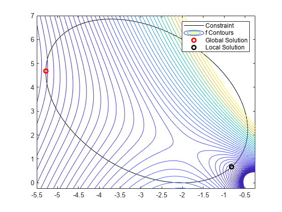

解位于非线性约束边界上。等高线图显示这些是仅有的局部最小值。该图还显示在 [–2,3/2] 附近存在一个平稳点，在 [–2,0] 和 [–1,4] 附近存在局部最大值。

Matlab求解函数

求解无约束极小值 

基于求解器求解

在matlab工具箱中，用于求解无约束极小值问题的函数有 fminunc 和 fminsearch （局部最优化算法）：

fminunc（采用拟牛顿法(QN)，是一种使用导数的算法）

[x, fval, exitflag, output, grad, hessian] = fminunc(fun, x0, options)

输入参数：

• fun 为要计算最小值的函数；
• x0 为初始点；
• options 为优化选项。

输出参数：

• x 为解，
• fval 为解处的目标函数值；
• exitflag 为fminunc 停止的原因，
• output 为有关优化过程的信息，
• grad 为解处的梯度，
• hessian 为逼近 Hessian 矩阵。

最小化函数：

fun = @(x)3*x(1)^2 + 2*x(1)*x(2) + x(2)^2 - 4*x(1) + 5*x(2);

调用 fminunc 以在 [1,1] 附近处求 fun 的最小值。

x0 = [1,1];
[x,fval] = fminunc(fun,x0)

Local minimum found.

Optimization completed because the size of the gradient is less than
the value of the optimality tolerance.

x = 1×2

    2.2500   -4.7500

fval = -16.3750

fminsearch（采用Nelder-Mead单纯形法，是一种直接搜索法）

[x, fval, exitflag, output, grad, hessian] = fminunc(fun, x0, options)

输入参数：

• fun 为要计算最小值的函数；
• x0 为初始点；
• options 为优化选项。

输出参数：

• x 为解，
• fval 为解处的目标函数值；
• exitflag 为fminunc 停止的原因，
• output 为有关优化过程的信息。

监视优化过程

options = optimset('PlotFcns',@optimplotfval);

将目标函数设置为 Rosenbrock 函数，

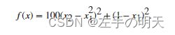
该函数的最小值在 x = [1,1] 处，最小值为 0。

将起始点设置为 x0 = [-1.2,1] 并使用 fminsearch 计算 Rosenbrock 函数的最小值。

fun = @(x)100*(x(2) - x(1)^2)^2 + (1 - x(1))^2;
x0 = [-1.2,1];
x = fminsearch(fun,x0,options)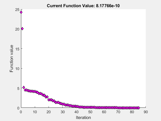

x = 1×2

    1.0000    1.0000

检查优化过程

在优化进行期间和优化结束后检查优化结果。

将选项设置为提供迭代输出，从而在求解器运行时提供有关优化的信息。此外，将绘图函数设置为在求解器运行时显示目标函数值。

options = optimset('Display','iter','PlotFcns',@optimplotfval);

设置目标函数和起始点。

function f = objectivefcn1(x)
f = 0;
for k = -10:10
    f = f + exp(-(x(1)-x(2))^2 - 2*x(1)^2)*cos(x(2))*sin(2*x(2));
end

将 objectivefcn1 的代码作为文件包含在路径中。

x0 = [0.25,-0.25];
fun = @objectivefcn1;

获取所有求解器输出。在求解器运行完毕后，使用这些输出检查结果。

[x,fval,exitflag,output] = fminsearch(fun,x0,options)

 
 Iteration   Func-count         f(x)         Procedure
     0            1         -6.70447         
     1            3         -6.89837         initial simplex
     2            5         -7.34101         expand
     3            7         -7.91894         expand
     4            9         -9.07939         expand
     5           11         -10.5047         expand
     6           13         -12.4957         expand
     7           15         -12.6957         reflect
     8           17         -12.8052         contract outside
     9           19         -12.8052         contract inside
    10           21         -13.0189         expand
    11           23         -13.0189         contract inside
    12           25         -13.0374         reflect
    13           27          -13.122         reflect
    14           28          -13.122         reflect
    15           29          -13.122         reflect
    16           31          -13.122         contract outside
    17           33         -13.1279         contract inside
    18           35         -13.1279         contract inside
    19           37         -13.1296         contract inside
    20           39         -13.1301         contract inside
    21           41         -13.1305         reflect
    22           43         -13.1306         contract inside
    23           45         -13.1309         contract inside
    24           47         -13.1309         contract inside
    25           49          -13.131         reflect
    26           51          -13.131         contract inside
    27           53          -13.131         contract inside
    28           55          -13.131         contract inside
    29           57          -13.131         contract outside
    30           59          -13.131         contract inside
    31           61          -13.131         contract inside
    32           63          -13.131         contract inside
    33           65          -13.131         contract outside
    34           67          -13.131         contract inside
    35           69          -13.131         contract inside
 
Optimization terminated:
 the current x satisfies the termination criteria using OPTIONS.TolX of 1.000000e-04 
 and F(X) satisfies the convergence criteria using OPTIONS.TolFun of 1.000000e-04 

x =

   -0.1696   -0.5086


fval =

  -13.1310


exitflag =

     1


output = 

  struct with fields:

    iterations: 35
     funcCount: 69
     algorithm: 'Nelder-Mead simplex direct search'
       message: 'Optimization terminated:...'

exitflag 的值为 1，这意味着 fminsearch 很可能收敛于局部最小值。

output 结构体显示迭代数。迭代输出中和绘图中也显示此信息。output 结构体还显示函数求值的次数，迭代输出方式会显示该次数，但所选的绘图函数不显示该次数。

基于问题求解

（1）基于求解器求解

clc, clear
f=@(x) x(1)^3-x(2)^3+3*x(1)^2+3*x(2)^2-9*x(1); 
g=@(x) -f(x);
[xy1,z1]=fminunc(f, rand(2,1))  %求极小值点
[xy2,z2]=fminsearch(g,rand(2,1)); %求极大值点
xy2, z2=-z2  %显示极大点及对应的极大值

（2）基于问题求解

clc, clear, prob1=optimproblem;  %最小值问题
x=optimvar('x','LowerBound',-3,'UpperBound',3);
y=optimvar('y','LowerBound',-4,'UpperBound',4);
prob1.Objective=x^3-y^3+3*x^2+3*y^2-9*x;
x0.x=1; x0.y=1;
[sol1,fval1,flag1,out1]=solve(prob1,x0)
prob2=optimproblem('ObjectiveSense','max')
prob2.Objective=x^3-y^3+3*x^2+3*y^2-9*x;
op=optimoptions(@fmincon,'Algorithm','active-set')
[sol2,fval2,flag2,out2]=solve(prob2,x0,'Options',op)

求得的极小值点为 (1，0)，极小值为 -5；极大值点为 (-3，2)，极大值为 31。

求解有约束极小值

基于求解器求解

非线性规划模型的一般形式为

b 和 beq 是向量，A 和 Aeq 是矩阵，c(x) 和 ceq(x) 是返回向量的函数，f(x) 是返回标量的函数。f(x)、c(x) 和 ceq(x) 可以是非线性函数。

x、lb 和 ub 可以作为向量或矩阵传递。

fmincon（寻找约束非线性多变量函数的最小值）

[x,fval,exitflag,output,lambda,grad,hessian] = fmincon(fun,x0,A,b,Aeq,beq,lb,ub,nonlcon,options)

输入参数：

• fun 为要计算最小值的函数
• x0 为初始点，指定为实数向量或实数数组。求解器使用 x0 的大小以及其中的元素数量确定 fun 接受的变量数量和大小。
• A 为线性不等式约束矩阵，A 表示约束中的线性系数；
• b 为线性不等式约束向量，b 表示约束中的常向量；
• Aeq 为线性等式约束矩阵，beq 为线性等式约束向量；
• lb 为下界，ub 为上界；
• nonlcon 为非线性约束；
• options 为 intlinprog 的选项，
• problem 为封装输入和选项的结构体，
• lambda 为解处的拉格朗日乘数，
• grad 为解处的梯度，
• hessian 为逼近 Hessian 矩阵

输出参数：

• x 为解
• fval 为目标函数最优值；
• exitflag 为算法停止条件，
• output 为求解过程摘要。

 在非线性约束下求函数的最小值

在边界约束下求 Rosenbrock 函数在圆内最小的点。

fun = @(x)100*(x(2)-x(1)^2)^2 + (1-x(1))^2;

在区域 

 内寻找。

lb = [0,0.2];
ub = [0.5,0.8];

同时在以 [1/3,1/3] 为圆心、半径为 1/3 的圆内寻找。

function [c,ceq] = circlecon(x)
c = (x(1)-1/3)^2 + (x(2)-1/3)^2 - (1/3)^2;
ceq = [];

没有线性约束，因此将这些参数设置为 []。

A = [];
b = [];
Aeq = [];
beq = [];

选择一个满足所有约束的初始点。

x0 = [1/4,1/4];

求解。

nonlcon = @circlecon;
x = fmincon(fun,x0,A,b,Aeq,beq,lb,ub,nonlcon)

Local minimum found that satisfies the constraints.

Optimization completed because the objective function is non-decreasing in 
feasible directions, to within the value of the optimality tolerance,
and constraints are satisfied to within the value of the constraint tolerance.


x =

    0.5000    0.2500

基于问题求解

（1）基于求解器求解

clc, clear
fun1 = @(x) sum(x.^2)+8;
[x,y]=fmincon(fun1,rand(3,1),[],[],[],[],zeros(3,1),[],@fun2)

function [c,ceq]=fun2(x)
c=[-x(1)^2+x(2)-x(3)^2
x(1)+x(2)^2+x(3)^3-20];  %非线性不等式约束
ceq=[-x(1)-x(2)^2+2
x(2)+2*x(3)^2-3]; %非线性等式约束
end

（2）基于问题求解

clc, clear, prob = optimproblem;
x = optimvar('x',3,'LowerBound',0);
prob.Objective = sum(x.^2)+8;
con1 = [-x(1)^2+x(2)-x(3)^2 <= 0
x(1)+x(2)^2+x(3)^3 <= 20];  %非线性不等式约束
con2 = [-x(1)-x(2)^2+2 == 0
         x(2)+2*x(3)^2 == 3]; %非线性等式约束
prob.Constraints.con1 = con1;
prob.Constraints.con2 = con2;
x0.x=rand(3,1);  %非线性规划必须赋初值
[sol,fval,flag,out]= solve(prob,x0), sol.x

求得当 x1 = 0.5522, x2 = 1.2033, x3 = 0.9478 时，最小值 y = 10.6511。