- 机器学习与深度学习间关系与区别
ℒℴѵℯ心·动ꦿ໊ོ꫞
人工智能学习深度学习python
一、机器学习概述定义机器学习(MachineLearning,ML)是一种通过数据驱动的方法,利用统计学和计算算法来训练模型,使计算机能够从数据中学习并自动进行预测或决策。机器学习通过分析大量数据样本,识别其中的模式和规律,从而对新的数据进行判断。其核心在于通过训练过程,让模型不断优化和提升其预测准确性。主要类型1.监督学习(SupervisedLearning)监督学习是指在训练数据集中包含输入
- Goolge earth studio 进阶4——路径修改与平滑
陟彼高冈yu
Googleearthstudio进阶教程旅游
如果我们希望在大约中途时获得更多的城市鸟瞰视角。可以将相机拖动到这里并创建一个新的关键帧。camera_target_clip_7EarthStudio会自动平滑我们的路径,所以当我们通过这个关键帧时,不是一个生硬的角度,而是一个平滑的曲线。camera_target_clip_8路径上有贝塞尔控制手柄,允许我们调整路径的形状。右键单击,我们可以选择“平滑路径”,这是默认的自动平滑算法,或者我们可
- 基于社交网络算法优化的二维最大熵图像分割
智能算法研学社(Jack旭)
智能优化算法应用图像分割算法php开发语言
智能优化算法应用:基于社交网络优化的二维最大熵图像阈值分割-附代码文章目录智能优化算法应用:基于社交网络优化的二维最大熵图像阈值分割-附代码1.前言2.二维最大熵阈值分割原理3.基于社交网络优化的多阈值分割4.算法结果:5.参考文献:6.Matlab代码摘要:本文介绍基于最大熵的图像分割,并且应用社交网络算法进行阈值寻优。1.前言阅读此文章前,请阅读《图像分割:直方图区域划分及信息统计介绍》htt
- 高端密码学院笔记285
柚子_b4b4
高端幸福密码学院(高级班)幸福使者:李华第(598)期《幸福》之回归内在深层生命原动力基础篇——揭秘“激励”成长的喜悦心理案例分析主讲:刘莉一,知识扩充:成功=艰苦劳动+正确方法+少说空话。贪图省力的船夫,目标永远下游。智者的梦再美,也不如愚人实干的脚印。幸福早课堂2020.10.16星期五一笔记:1,重视和珍惜的前提是知道它的价值非常重要,当你珍惜了,你就真正定下来,真正的学到身上。2,大家需要
- 121. 买卖股票的最佳时机
薄荷糖的味道_fb40
给定一个数组,它的第i个元素是一支给定股票第i天的价格。如果你最多只允许完成一笔交易(即买入和卖出一支股票),设计一个算法来计算你所能获取的最大利润。注意你不能在买入股票前卖出股票。示例1:输入:[7,1,5,3,6,4]输出:5解释:在第2天(股票价格=1)的时候买入,在第5天(股票价格=6)的时候卖出,最大利润=6-1=5。注意利润不能是7-1=6,因为卖出价格需要大于买入价格。示例2:输入:
- 每日算法&面试题,大厂特训二十八天——第二十天(树)
肥学
⚡算法题⚡面试题每日精进java算法数据结构
目录标题导读算法特训二十八天面试题点击直接资料领取导读肥友们为了更好的去帮助新同学适应算法和面试题,最近我们开始进行专项突击一步一步来。上一期我们完成了动态规划二十一天现在我们进行下一项对各类算法进行二十八天的一个小总结。还在等什么快来一起肥学进行二十八天挑战吧!!特别介绍小白练手专栏,适合刚入手的新人欢迎订阅编程小白进阶python有趣练手项目里面包括了像《机器人尬聊》《恶搞程序》这样的有趣文章
- 回溯算法-重新安排行程
chirou_
算法数据结构图论c++图搜索
leetcode332.重新安排行程这题我还没自己ac过,只能现在凭着刚学完的热乎劲把我对题解的理解记下来。本题我认为对数据结构的考察比较多,用什么数据结构去存数据,去读取数据,都是很重要的。classSolution{private:unordered_map>targets;boolbacktracking(intticketNum,vector&result){//1.确定参数和返回值//2
- Faiss:高效相似性搜索与聚类的利器
网络·魚
大数据faiss
Faiss是一个针对大规模向量集合的相似性搜索库,由FacebookAIResearch开发。它提供了一系列高效的算法和数据结构,用于加速向量之间的相似性搜索,特别是在大规模数据集上。本文将介绍Faiss的原理、核心功能以及如何在实际项目中使用它。Faiss原理:近似最近邻搜索:Faiss的核心功能之一是近似最近邻搜索,它能够高效地在大规模数据集中找到与给定查询向量最相似的向量。这种搜索是近似的,
- 【华为OD技术面试真题 - 技术面】- python八股文真题题库(1)
算法大师
华为od面试python
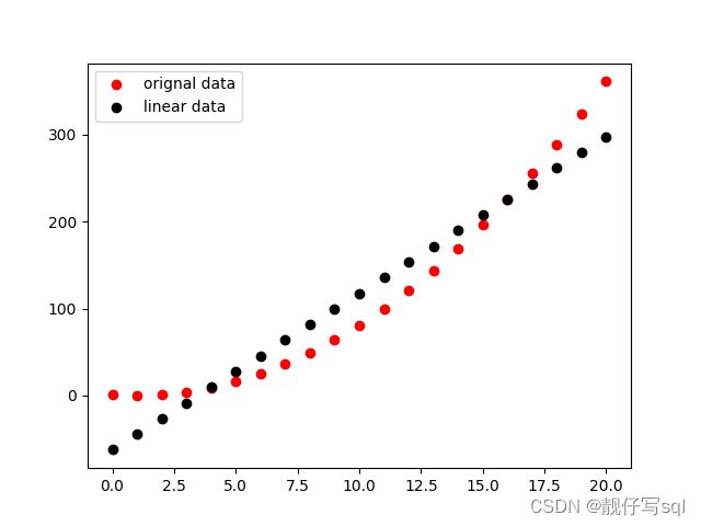
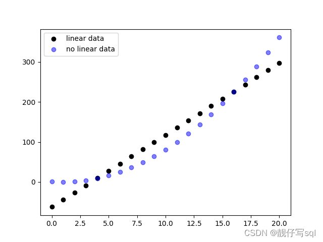
华为OD面试真题精选专栏:华为OD面试真题精选目录:2024华为OD面试手撕代码真题目录以及八股文真题目录文章目录华为OD面试真题精选1.数据预处理流程数据预处理的主要步骤工具和库2.介绍线性回归、逻辑回归模型线性回归(LinearRegression)模型形式:关键点:逻辑回归(LogisticRegression)模型形式:关键点:参数估计与评估:3.python浅拷贝及深拷贝浅拷贝(Shal
- insert into select 主键自增_mybatis拦截器实现主键自动生成
weixin_39521651
insertintoselect主键自增mybatisdelete返回值mybatisinsert返回主键mybatisinsert返回对象mybatisplusinsert返回主键mybatisplus插入生成id
前言前阵子和朋友聊天,他说他们项目有个需求,要实现主键自动生成,不想每次新增的时候,都手动设置主键。于是我就问他,那你们数据库表设置主键自动递增不就得了。他的回答是他们项目目前的id都是采用雪花算法来生成,因此为了项目稳定性,不会切换id的生成方式。朋友问我有没有什么实现思路,他们公司的orm框架是mybatis,我就建议他说,不然让你老大把mybatis切换成mybatis-plus。mybat
- k均值聚类算法考试例题_k均值算法(k均值聚类算法计算题)
寻找你83497
k均值聚类算法考试例题
?算法:第一步:选K个初始聚类中心,z1(1),z2(1),…,zK(1),其中括号内的序号为寻找聚类中心的迭代运算的次序号。聚类中心的向量值可任意设定,例如可选开始的K个.k均值聚类:---------一种硬聚类算法,隶属度只有两个取值0或1,提出的基本根据是“类内误差平方和最小化”准则;模糊的c均值聚类算法:--------一种模糊聚类算法,是.K均值聚类算法是先随机选取K个对象作为初始的聚类
- Python实现简单的机器学习算法
master_chenchengg
pythonpython办公效率python开发IT
Python实现简单的机器学习算法开篇:初探机器学习的奇妙之旅搭建环境:一切从安装开始必备工具箱第一步:安装Anaconda和JupyterNotebook小贴士:如何配置Python环境变量算法初体验:从零开始的Python机器学习线性回归:让数据说话数据准备:从哪里找数据编码实战:Python实现线性回归模型评估:如何判断模型好坏逻辑回归:从分类开始理论入门:什么是逻辑回归代码实现:使用skl
- 推荐算法_隐语义-梯度下降
_feivirus_
算法机器学习和数学推荐算法机器学习隐语义
importnumpyasnp1.模型实现"""inputrate_matrix:M行N列的评分矩阵,值为P*Q.P:初始化用户特征矩阵M*K.Q:初始化物品特征矩阵K*N.latent_feature_cnt:隐特征的向量个数max_iteration:最大迭代次数alpha:步长lamda:正则化系数output分解之后的P和Q"""defLFM_grad_desc(rate_matrix,l
- K近邻算法_分类鸢尾花数据集
_feivirus_
算法机器学习和数学分类机器学习K近邻
importnumpyasnpimportpandasaspdfromsklearn.datasetsimportload_irisfromsklearn.model_selectionimporttrain_test_splitfromsklearn.metricsimportaccuracy_score1.数据预处理iris=load_iris()df=pd.DataFrame(data=ir
- 数据结构 | 栈和队列
TT-Kun
数据结构与算法数据结构栈队列C语言
文章目录栈和队列1.栈:后进先出(LIFO)的数据结构1.1概念与结构1.2栈的实现2.队列:先进先出(FIFO)的数据结构2.1概念与结构2.2队列的实现3.栈和队列算法题3.1有效的括号3.2用队列实现栈3.3用栈实现队列3.4设计循环队列结论栈和队列在计算机科学中,栈和队列是两种基本且重要的数据结构,它们在处理数据存储和访问顺序方面有着独特的规则和应用。本文将详细介绍栈和队列的概念、结构、实
- [Python] 数据结构 详解及代码
AIAdvocate
算法python数据结构链表
今日内容大纲介绍数据结构介绍列表链表1.数据结构和算法简介程序大白话翻译,程序=数据结构+算法数据结构指的是存储,组织数据的方式.算法指的是为了解决实际业务问题而思考思路和方法,就叫:算法.2.算法的5大特性介绍算法具有独立性算法是解决问题的思路和方式,最重要的是思维,而不是语言,其(算法)可以通过多种语言进行演绎.5大特性有输入,需要传入1或者多个参数有输出,需要返回1个或者多个结果有穷性,执行
- Python算法L5:贪心算法
小熊同学哦
Python算法算法python贪心算法
Python贪心算法简介目录Python贪心算法简介贪心算法的基本步骤贪心算法的适用场景经典贪心算法问题1.**零钱兑换问题**2.**区间调度问题**3.**背包问题**贪心算法的优缺点优点:缺点:结语贪心算法(GreedyAlgorithm)是一种在每一步选择中都采取当前最优或最优解的算法。它的核心思想是,在保证每一步局部最优的情况下,希望通过贪心选择达到全局最优解。虽然贪心算法并不总能得到全
- 【RabbitMQ 项目】服务端:数据管理模块之绑定管理
月夜星辉雪
rabbitmq分布式
文章目录一.编写思路二.代码实践一.编写思路定义绑定信息类交换机名称队列名称绑定关键字:交换机的路由交换算法中会用到没有是否持久化的标志,因为绑定是否持久化取决于交换机和队列是否持久化,只有它们都持久化时绑定才需要持久化。绑定就好像一根绳子,两端连接着交换机和队列,当一方不存在,它就没有存在的必要了定义绑定持久化类构造函数:如果数据库文件不存在则创建,打开数据库,创建binding_table插入
- 非对称加密算法原理与应用2——RSA私钥加密文件
私语茶馆
云部署与开发架构及产品灵感记录RSA2048私钥加密
作者:私语茶馆1.相关章节(1)非对称加密算法原理与应用1——秘钥的生成-CSDN博客第一章节讲述的是创建秘钥对,并将公钥和私钥导出为文件格式存储。本章节继续讲如何利用私钥加密内容,包括从密钥库或文件中读取私钥,并用RSA算法加密文件和String。2.私钥加密的概述本文主要基于第一章节的RSA2048bit的非对称加密算法讲述如何利用私钥加密文件。这种加密后的文件,只能由该私钥对应的公钥来解密。
- 粒子群优化 (PSO) 在三维正弦波函数中的应用
subject625Ruben
机器学习人工智能matlab算法
在这篇博客中,我们将展示如何使用粒子群优化(PSO)算法求解三维正弦波函数,并通过增加正弦波扰动,使优化过程更加复杂和有趣。本文将介绍目标函数的定义、PSO参数设置以及算法执行的详细过程,并展示搜索空间中的动态过程和收敛曲线。1.目标函数定义我们使用的目标函数是一个三维正弦波函数,定义如下:objectiveFunc=@(x)sin(sqrt(x(1).^2+x(2).^2))+0.5*sin(5
- 非对称加密算法————RSA理论及详情
hu19930613
转自:https://www.kancloud.cn/kancloud/rsa_algorithm/48484一、一点历史1976年以前,所有的加密方法都是同一种模式:(1)甲方选择某一种加密规则,对信息进行加密;(2)乙方使用同一种规则,对信息进行解密。由于加密和解密使用同样规则(简称"密钥"),这被称为"对称加密算法"(Symmetric-keyalgorithm)。这种加密模式有一个最大弱点
- ai绘画工具midjourney怎么下载?附作品管理教程
设计师早上好
Midjourney是一款功能强大的AI绘画工具,它使用机器学习技术和深度神经网络等算法,可以生成各种艺术风格的绘画作品。在创意设计、广告宣传等方面有着广泛的应用前景。那么,ai绘画工具midjourney怎么下载?本文将为您介绍Midjourney的下载以及作品的相关管理。一、Midjourney下载Midjourney的下载非常简单,只需打开Midjourney官网(点击“GetMidjour
- 【加密算法基础——对称加密和非对称加密】
XWWW668899
网络安全服务器笔记
对称加密与非对称加密对称加密和非对称加密是两种基本的加密方法,各自有不同的特点和用途。以下是详细比较:1.对称加密特点密钥:使用相同的密钥进行加密和解密。发送方和接收方必须共享这个密钥。速度:通常速度较快,适合处理大量数据。实现:算法相对简单,计算效率高。常见算法AES(高级加密标准)DES(数据加密标准)3DES(三重数据加密标准)RC4(流密码)应用场景文件加密磁盘加密传输大量数据时的加密2.
- 【算法练习】IDEA集成leetcode插件实现快速刷
2401_84102892
2024年程序员学习算法intellij-idealeetcode
============点击右侧边leetcode->设置->配置地址、用户名、密码、存放目录、文件模板用户名要登录后在账号信息里看模板代码1.codefilename!velocityTool.camelC
- [实践应用] 深度学习之模型性能评估指标
YuanDaima2048
深度学习工具使用深度学习人工智能损失函数性能评估pytorchpython机器学习
文章总览:YuanDaiMa2048博客文章总览深度学习之模型性能评估指标分类任务回归任务排序任务聚类任务生成任务其他介绍在机器学习和深度学习领域,评估模型性能是一项至关重要的任务。不同的学习任务需要不同的性能指标来衡量模型的有效性。以下是对一些常见任务及其相应的性能评估指标的详细解释和总结。分类任务分类任务是指模型需要将输入数据分配到预定义的类别或标签中。以下是分类任务中常用的性能指标:准确率(
- 【加密算法基础——RSA 加密】
XWWW668899
网络服务器笔记python
RSA加密RSA(Rivest-Shamir-Adleman)加密是非对称加密,一种广泛使用的公钥加密算法,主要用于安全数据传输。公钥用于加密,私钥用于解密。RSA加密算法的名称来源于其三位发明者的姓氏:R:RonRivestS:AdiShamirA:LeonardAdleman这三位计算机科学家在1977年共同提出了这一算法,并发表了相关论文。他们的工作为公钥加密的基础奠定了重要基础,使得安全通
- 机器学习-聚类算法
不良人龍木木
机器学习机器学习算法聚类
机器学习-聚类算法1.AHC2.K-means3.SC4.MCL仅个人笔记,感谢点赞关注!1.AHC2.K-means3.SC传统谱聚类:个人对谱聚类算法的理解以及改进4.MCL目前仅专注于NLP的技术学习和分享感谢大家的关注与支持!
- 生成式地图制图
Bwywb_3
深度学习机器学习深度学习生成对抗网络
生成式地图制图(GenerativeCartography)是一种利用生成式算法和人工智能技术自动创建地图的技术。它结合了传统的地理信息系统(GIS)技术与现代生成模型(如深度学习、GANs等),能够根据输入的数据自动生成符合需求的地图。这种方法在城市规划、虚拟环境设计、游戏开发等多个领域具有应用前景。主要特点:自动化生成:通过算法和模型,系统能够根据输入的地理或空间数据自动生成地图,而无需人工逐
- 高性能javascript--算法和流程控制
海淀萌狗
-for,while和do-while性能相当-避免使用for-in循环,==除非遍历一个属性量未知的对象==es5:for-in遍历的对象便不局限于数组,还可以遍历对象。原因:for-in每次迭代操作会同时搜索实例或者原型属性,for-in循环的每次迭代都会产生更多开销,因此要比其他循环类型慢,一般速度为其他类型循环的1/7。因此,除非明确需要迭代一个属性数量未知的对象,否则应避免使用for-i
- 深度 Qlearning:在直播推荐系统中的应用
AGI通用人工智能之禅
程序员提升自我硅基计算碳基计算认知计算生物计算深度学习神经网络大数据AIGCAGILLMJavaPython架构设计Agent程序员实现财富自由
深度Q-learning:在直播推荐系统中的应用关键词:深度Q-learning,强化学习,直播推荐系统,个性化推荐1.背景介绍1.1问题的由来随着互联网技术的飞速发展,直播平台如雨后春笋般涌现。面对海量的直播内容,用户很难快速找到自己感兴趣的内容。因此,个性化推荐系统在直播平台中扮演着越来越重要的角色。1.2研究现状目前,主流的个性化推荐算法包括协同过滤、基于内容的推荐等。这些方法在一定程度上缓
- ViewController添加button按钮解析。(翻译)
张亚雄
c
<div class="it610-blog-content-contain" style="font-size: 14px"></div>// ViewController.m
// Reservation software
//
// Created by 张亚雄 on 15/6/2.
- mongoDB 简单的增删改查
开窍的石头
mongodb
在上一篇文章中我们已经讲了mongodb怎么安装和数据库/表的创建。在这里我们讲mongoDB的数据库操作
在mongo中对于不存在的表当你用db.表名 他会自动统计
下边用到的user是表明,db代表的是数据库
添加(insert):
- log4j配置
0624chenhong
log4j
1) 新建java项目
2) 导入jar包,项目右击,properties—java build path—libraries—Add External jar,加入log4j.jar包。
3) 新建一个类com.hand.Log4jTest
package com.hand;
import org.apache.log4j.Logger;
public class
- 多点触摸(图片缩放为例)
不懂事的小屁孩
多点触摸
多点触摸的事件跟单点是大同小异的,上个图片缩放的代码,供大家参考一下
import android.app.Activity;
import android.os.Bundle;
import android.view.MotionEvent;
import android.view.View;
import android.view.View.OnTouchListener
- 有关浏览器窗口宽度高度几个值的解析
换个号韩国红果果
JavaScripthtml
1 元素的 offsetWidth 包括border padding content 整体的宽度。
clientWidth 只包括内容区 padding 不包括border。
clientLeft = offsetWidth -clientWidth 即这个元素border的值
offsetLeft 若无已定位的包裹元素
- 数据库产品巡礼:IBM DB2概览
蓝儿唯美
db2
IBM DB2是一个支持了NoSQL功能的关系数据库管理系统,其包含了对XML,图像存储和Java脚本对象表示(JSON)的支持。DB2可被各种类型的企 业使用,它提供了一个数据平台,同时支持事务和分析操作,通过提供持续的数据流来保持事务工作流和分析操作的高效性。 DB2支持的操作系统
DB2可应用于以下三个主要的平台:
工作站,DB2可在Linus、Unix、Windo
- java笔记5
a-john
java
控制执行流程:
1,true和false
利用条件表达式的真或假来决定执行路径。例:(a==b)。它利用条件操作符“==”来判断a值是否等于b值,返回true或false。java不允许我们将一个数字作为布尔值使用,虽然这在C和C++里是允许的。如果想在布尔测试中使用一个非布尔值,那么首先必须用一个条件表达式将其转化成布尔值,例如if(a!=0)。
2,if-els
- Web开发常用手册汇总
aijuans
PHP
一门技术,如果没有好的参考手册指导,很难普及大众。这其实就是为什么很多技术,非常好,却得不到普遍运用的原因。
正如我们学习一门技术,过程大概是这个样子:
①我们日常工作中,遇到了问题,困难。寻找解决方案,即寻找新的技术;
②为什么要学习这门技术?这门技术是不是很好的解决了我们遇到的难题,困惑。这个问题,非常重要,我们不是为了学习技术而学习技术,而是为了更好的处理我们遇到的问题,才需要学习新的
- 今天帮助人解决的一个sql问题
asialee
sql
今天有个人问了一个问题,如下:
type AD value
A
- 意图对象传递数据
百合不是茶
android意图IntentBundle对象数据的传递
学习意图将数据传递给目标活动; 初学者需要好好研究的
1,将下面的代码添加到main.xml中
<?xml version="1.0" encoding="utf-8"?>
<LinearLayout xmlns:android="http:/
- oracle查询锁表解锁语句
bijian1013
oracleobjectsessionkill
一.查询锁定的表
如下语句,都可以查询锁定的表
语句一:
select a.sid,
a.serial#,
p.spid,
c.object_name,
b.session_id,
b.oracle_username,
b.os_user_name
from v$process p, v$s
- mac osx 10.10 下安装 mysql 5.6 二进制文件[tar.gz]
征客丶
mysqlosx
场景:在 mac osx 10.10 下安装 mysql 5.6 的二进制文件。
环境:mac osx 10.10、mysql 5.6 的二进制文件
步骤:[所有目录请从根“/”目录开始取,以免层级弄错导致找不到目录]
1、下载 mysql 5.6 的二进制文件,下载目录下面称之为 mysql5.6SourceDir;
下载地址:http://dev.mysql.com/downl
- 分布式系统与框架
bit1129
分布式
RPC框架 Dubbo
什么是Dubbo
Dubbo是一个分布式服务框架,致力于提供高性能和透明化的RPC远程服务调用方案,以及SOA服务治理方案。其核心部分包含: 远程通讯: 提供对多种基于长连接的NIO框架抽象封装,包括多种线程模型,序列化,以及“请求-响应”模式的信息交换方式。 集群容错: 提供基于接
- 那些令人蛋痛的专业术语
白糖_
springWebSSOIOC
spring
【控制反转(IOC)/依赖注入(DI)】:
由容器控制程序之间的关系,而非传统实现中,由程序代码直接操控。这也就是所谓“控制反转”的概念所在:控制权由应用代码中转到了外部容器,控制权的转移,是所谓反转。
简单的说:对象的创建又容器(比如spring容器)来执行,程序里不直接new对象。
Web
【单点登录(SSO)】:SSO的定义是在多个应用系统中,用户
- 《给大忙人看的java8》摘抄
braveCS
java8
函数式接口:只包含一个抽象方法的接口
lambda表达式:是一段可以传递的代码
你最好将一个lambda表达式想象成一个函数,而不是一个对象,并记住它可以被转换为一个函数式接口。
事实上,函数式接口的转换是你在Java中使用lambda表达式能做的唯一一件事。
方法引用:又是要传递给其他代码的操作已经有实现的方法了,这时可以使
- 编程之美-计算字符串的相似度
bylijinnan
java算法编程之美
public class StringDistance {
/**
* 编程之美 计算字符串的相似度
* 我们定义一套操作方法来把两个不相同的字符串变得相同,具体的操作方法为:
* 1.修改一个字符(如把“a”替换为“b”);
* 2.增加一个字符(如把“abdd”变为“aebdd”);
* 3.删除一个字符(如把“travelling”变为“trav
- 上传、下载压缩图片
chengxuyuancsdn
下载
/**
*
* @param uploadImage --本地路径(tomacat路径)
* @param serverDir --服务器路径
* @param imageType --文件或图片类型
* 此方法可以上传文件或图片.txt,.jpg,.gif等
*/
public void upload(String uploadImage,Str
- bellman-ford(贝尔曼-福特)算法
comsci
算法F#
Bellman-Ford算法(根据发明者 Richard Bellman 和 Lester Ford 命名)是求解单源最短路径问题的一种算法。单源点的最短路径问题是指:给定一个加权有向图G和源点s,对于图G中的任意一点v,求从s到v的最短路径。有时候这种算法也被称为 Moore-Bellman-Ford 算法,因为 Edward F. Moore zu 也为这个算法的发展做出了贡献。
与迪科
- oracle ASM中ASM_POWER_LIMIT参数
daizj
ASMoracleASM_POWER_LIMIT磁盘平衡
ASM_POWER_LIMIT
该初始化参数用于指定ASM例程平衡磁盘所用的最大权值,其数值范围为0~11,默认值为1。该初始化参数是动态参数,可以使用ALTER SESSION或ALTER SYSTEM命令进行修改。示例如下:
SQL>ALTER SESSION SET Asm_power_limit=2;
- 高级排序:快速排序
dieslrae
快速排序
public void quickSort(int[] array){
this.quickSort(array, 0, array.length - 1);
}
public void quickSort(int[] array,int left,int right){
if(right - left <= 0
- C语言学习六指针_何谓变量的地址 一个指针变量到底占几个字节
dcj3sjt126com
C语言
# include <stdio.h>
int main(void)
{
/*
1、一个变量的地址只用第一个字节表示
2、虽然他只使用了第一个字节表示,但是他本身指针变量类型就可以确定出他指向的指针变量占几个字节了
3、他都只存了第一个字节地址,为什么只需要存一个字节的地址,却占了4个字节,虽然只有一个字节,
但是这些字节比较多,所以编号就比较大,
- phpize使用方法
dcj3sjt126com
PHP
phpize是用来扩展php扩展模块的,通过phpize可以建立php的外挂模块,下面介绍一个它的使用方法,需要的朋友可以参考下
安装(fastcgi模式)的时候,常常有这样一句命令:
代码如下:
/usr/local/webserver/php/bin/phpize
一、phpize是干嘛的?
phpize是什么?
phpize是用来扩展php扩展模块的,通过phpi
- Java虚拟机学习 - 对象引用强度
shuizhaosi888
JAVA虚拟机
本文原文链接:http://blog.csdn.net/java2000_wl/article/details/8090276 转载请注明出处!
无论是通过计数算法判断对象的引用数量,还是通过根搜索算法判断对象引用链是否可达,判定对象是否存活都与“引用”相关。
引用主要分为 :强引用(Strong Reference)、软引用(Soft Reference)、弱引用(Wea
- .NET Framework 3.5 Service Pack 1(完整软件包)下载地址
happyqing
.net下载framework
Microsoft .NET Framework 3.5 Service Pack 1(完整软件包)
http://www.microsoft.com/zh-cn/download/details.aspx?id=25150
Microsoft .NET Framework 3.5 Service Pack 1 是一个累积更新,包含很多基于 .NET Framewo
- JAVA定时器的使用
jingjing0907
javatimer线程定时器
1、在应用开发中,经常需要一些周期性的操作,比如每5分钟执行某一操作等。
对于这样的操作最方便、高效的实现方式就是使用java.util.Timer工具类。
privatejava.util.Timer timer;
timer = newTimer(true);
timer.schedule(
newjava.util.TimerTask() { public void run()
- Webbench
流浪鱼
webbench
首页下载地址 http://home.tiscali.cz/~cz210552/webbench.html
Webbench是知名的网站压力测试工具,它是由Lionbridge公司(http://www.lionbridge.com)开发。
Webbench能测试处在相同硬件上,不同服务的性能以及不同硬件上同一个服务的运行状况。webbench的标准测试可以向我们展示服务器的两项内容:每秒钟相
- 第11章 动画效果(中)
onestopweb
动画
index.html
<!DOCTYPE html PUBLIC "-//W3C//DTD XHTML 1.0 Transitional//EN" "http://www.w3.org/TR/xhtml1/DTD/xhtml1-transitional.dtd">
<html xmlns="http://www.w3.org/
- windows下制作bat启动脚本.
sanyecao2314
javacmd脚本bat
java -classpath C:\dwjj\commons-dbcp.jar;C:\dwjj\commons-pool.jar;C:\dwjj\log4j-1.2.16.jar;C:\dwjj\poi-3.9-20121203.jar;C:\dwjj\sqljdbc4.jar;C:\dwjj\voucherimp.jar com.citsamex.core.startup.MainStart
- Java进行RSA加解密的例子
tomcat_oracle
java
加密是保证数据安全的手段之一。加密是将纯文本数据转换为难以理解的密文;解密是将密文转换回纯文本。 数据的加解密属于密码学的范畴。通常,加密和解密都需要使用一些秘密信息,这些秘密信息叫做密钥,将纯文本转为密文或者转回的时候都要用到这些密钥。 对称加密指的是发送者和接收者共用同一个密钥的加解密方法。 非对称加密(又称公钥加密)指的是需要一个私有密钥一个公开密钥,两个不同的密钥的
- Android_ViewStub
阿尔萨斯
ViewStub
public final class ViewStub extends View
java.lang.Object
android.view.View
android.view.ViewStub
类摘要: ViewStub 是一个隐藏的,不占用内存空间的视图对象,它可以在运行时延迟加载布局资源文件。当 ViewSt