一些经典的神经网络（第17天）

1. 经典神经网络LeNet

LeNet是早期成功的神经网络；
先使用卷积层来学习图片空间信息
然后使用全连接层来转到到类别空间

【通过在卷积层后加入激活函数，可以引入非线性、增加模型的表达能力、增强稀疏性和解决梯度消失等问题，从而提高卷积神经网络的性能和效果】

LeNet由两部分组成：卷积编码器和全连接层密集块

import torch
from torch import nn
from d2l import torch as d2l

class Reshape(torch.nn.Module):
    def forward(self, x):
        return x.view(-1, 1, 28, 28) # 批量数不变，通道数=1，h=28, w=28

net = torch.nn.Sequential(Reshape(), 
                          nn.Conv2d(1, 6, kernel_size=5, padding=2), nn.Sigmoid(), # 在卷积后加激活函数，填充是因为原始处理数据是32*32
                          nn.AvgPool2d(kernel_size=2, stride=2), # 池化层
                          nn.Conv2d(6, 16, kernel_size=5), nn.Sigmoid(),
                          nn.AvgPool2d(kernel_size=2, stride=2), 
                          nn.Flatten(), # 将4D结果拉成向量
                          # 相当于两个隐藏层的MLP
                          nn.Linear(16 * 5 * 5, 120), nn.Sigmoid(),
                          nn.Linear(120, 84), nn.Sigmoid(), 
                          nn.Linear(84, 10))

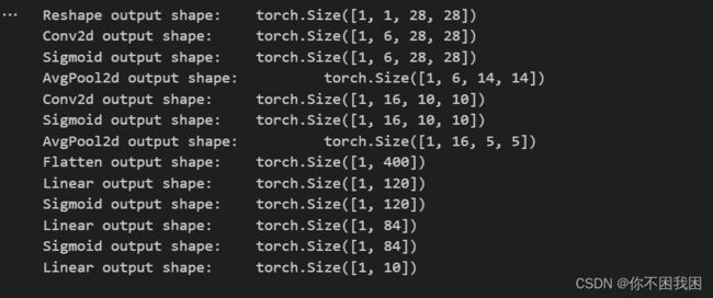
检查模型

X = torch.rand(size=(1, 1, 28, 28), dtype=torch.float32)
for layer in net:
    X = layer(X) 
    """
    对神经网络 net 中的每一层进行迭代，并打印每一层的输出形状
    layer.__class__.__name__ 是获取当前层的类名，即层的类型
    """
    print(layer.__class__.__name__, 'output shape: \t', X.shape)

LeNet在Fashion-MNIST数据集上的表现

batch_size = 256
train_iter, test_iter = d2l.load_data_fashion_mnist(batch_size=batch_size)

# 对evaluate_accuarcy函数进行轻微的修改
def evaluate_accuracy_gpu(net, data_iter, device=None):  
    """使用GPU计算模型在数据集上的精度。"""
    if isinstance(net, torch.nn.Module):
        net.eval()
        if not device:
            device = next(iter(net.parameters())).device
    metric = d2l.Accumulator(2)
    for X, y in data_iter:
        if isinstance(X, list):
            X = [x.to(device) for x in X]
        else:
            X = X.to(device)
        y = y.to(device)
        metric.add(d2l.accuracy(net(X), y), y.numel())
    return metric[0] / metric[1]  # 分类正确的个数 / 总个数

【
net.to(device) 是将神经网络 net 中的所有参数和缓冲区移动到指定的设备上进行计算的操作。

net 是一个神经网络模型。device 是指定的设备，可以是 torch.device 对象，如 torch.device(‘cuda’) 表示将模型移动到 GPU 上进行计算，或者是字符串，如 ‘cuda:0’ 表示将模型移动到指定编号的 GPU 上进行计算，也可以是 ‘cpu’ 表示将模型移动到 CPU 上进行计算。
通过调用 net.to(device)，模型中的所有参数和缓冲区将被复制到指定的设备上，并且之后的计算将在该设备上进行。这样可以利用 GPU 的并行计算能力来加速模型训练和推断过程。
注意，仅仅调用 net.to(device) 并不会对输入数据进行迁移，需要手动将输入数据也移动到相同的设备上才能与模型进行计算。例如，可以使用 input = input.to(device) 将输入数据 input 移动到指定设备上。】

# 为了使用 GPU，我们还需要一点小改动
def train_ch6(net, train_iter, test_iter, num_epochs, lr, device):
    """用GPU训练模型(在第六章定义)。"""
    def init_weights(m): # 初始化权重
        if type(m) == nn.Linear or type(m) == nn.Conv2d: 
            nn.init.xavier_uniform_(m.weight)

    net.apply(init_weights) # 对整个网络应用初始化
    print('training on', device)
    net.to(device) # 将神经网络 net 中的所有参数和缓冲区移动到指定的设备上进行计算的操作
    optimizer = torch.optim.SGD(net.parameters(), lr=lr) # 定义优化器
    loss = nn.CrossEntropyLoss() # 定义损失函数
    # 动画效果
    animator = d2l.Animator(xlabel='epoch', xlim=[1, num_epochs],
                            legend=['train loss', 'train acc', 'test acc'])
    timer, num_batches = d2l.Timer(), len(train_iter)

    for epoch in range(num_epochs):
        metric = d2l.Accumulator(3) # metric被初始化为存储3个指标值的累加器
        net.train()
        for i, (X, y) in enumerate(train_iter):
            timer.start()
            optimizer.zero_grad()
            # 将输入输出数据也移动到相同的设备
            X, y = X.to(device), y.to(device)
            y_hat = net(X)
            l = loss(y_hat, y)
            l.backward()
            optimizer.step()
            with torch.no_grad():
                metric.add(l * X.shape[0], d2l.accuracy(y_hat, y), X.shape[0])
            timer.stop()
            train_l = metric[0] / metric[2]
            train_acc = metric[1] / metric[2]
            # 动画效果
            if (i + 1) % (num_batches // 5) == 0 or i == num_batches - 1:
                animator.add(epoch + (i + 1) / num_batches,
                             (train_l, train_acc, None))
        test_acc = evaluate_accuracy_gpu(net, test_iter)
        animator.add(epoch + 1, (None, None, test_acc))
    print(f'loss {train_l:.3f}, train acc {train_acc:.3f}, '
          f'test acc {test_acc:.3f}')
    print(f'{metric[2] * num_epochs / timer.sum():.1f} examples/sec '
          f'on {str(device)}')

训练和评估LeNet-5模型

lr, num_epochs = 0.9, 10
train_ch6(net, train_iter, test_iter, num_epochs, lr, d2l.try_gpu())

2. 深度卷积神经网络（AlexNet）

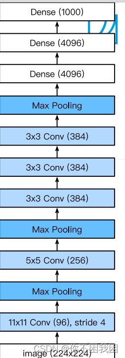
AlexNet架构 VS LeNet：
更大的核窗口和步长，因为图片更大了
更大的池化窗口，使用maxpooling
更多的输出通道
添加了3层卷积层
更多的输出

更多细节：

• 激活函数从sigmod变成了Rel（减缓梯度消失)
• 隐藏全连接层后加入了丢弃层dropout
• 数据增强

总结：

• AlexNet是更大更深的LeNet，处理的参数个数和计算复杂度大幅度提升
• 新加入了丢弃法,ReLU激活函数，最大池化层和数据增强

代码实现：

import torch
from torch import nn
from d2l import torch as d2l

net = nn.Sequential(
    nn.Conv2d(1, 96, kernel_size=11, stride=4, padding=1), nn.ReLU(), # 在MNIST输入通道是1，在ImageNet测试集上输入为3
    nn.MaxPool2d(kernel_size=3, stride=2),
    nn.Conv2d(96, 256, kernel_size=5, padding=2), nn.ReLU(), # 相比于LeNet将激活函数改为ReLU
    nn.MaxPool2d(kernel_size=3, stride=2),
    nn.Conv2d(256, 384, kernel_size=3, padding=1), nn.ReLU(),
    nn.Conv2d(384, 384, kernel_size=3, padding=1), nn.ReLU(),
    nn.Conv2d(384, 256, kernel_size=3, padding=1), nn.ReLU(),
    nn.MaxPool2d(kernel_size=3, stride=2), 
    nn.Flatten(), # 将4D->2D
    nn.Linear(6400, 4096), nn.ReLU(), nn.Dropout(p=0.5), # 添加丢弃
    nn.Linear(4096, 4096), nn.ReLU(), nn.Dropout(p=0.5),
    nn.Linear(4096, 10)) # 在Fashion-MNIST上做测试所以输出为10

# 构造一个单通道数据，来观察每一层输出的形状
X = torch.randn(1, 1, 224, 224)
for layer in net:
    X = layer(X)
    print(layer.__class__.__name__, 'Output shape:\t', X.shape)

# Fashion-MNIST图像的分辨率低于ImageNet图像，所以将其增加到224x224
batch_size = 128
train_iter, test_iter = d2l.load_data_fashion_mnist(batch_size, resize=224)
# 训练AlexNet
lr, num_epochs = 0.01, 10
d2l.train_ch6(net, train_iter, test_iter, num_epochs, lr, d2l.try_gpu())