Udacity机器人软件工程师课程笔记（二十二) - 物体识别 - 色彩直方图，支持向量机SVM

物体识别

1.HSV色彩空间

如果要进行颜色检测，HSV颜色空间是当前最常用的。

HSV(Hue, Saturation, Value)是根据颜色的直观特性由A. R. Smith在1978年创建的一种颜色空间, 也称六角锥体模型(Hexcone Model)。这个模型中颜色的参数分别是：色调（H），饱和度（S），亮度（V）。

HSV模型的三维表示从RGB立方体演化而来。设想从RGB沿立方体对角线的白色顶点向黑色顶点观察，就可以看到立方体的六边形外形。六边形边界表示色彩，水平轴表示纯度，明度沿垂直轴测量。

2.颜色直方图

使用生成的点云，将需要为3D空间中找到的点构造颜色直方图。但是，出于示例练习的目的，对2D图像中的像素进行操作就足够了。

首先我们先输出RGB图像的直方图，程序如下:

import matplotlib.image as mpimg
import matplotlib.pyplot as plt
import numpy as np

# 载入图片
image = mpimg.imread('hsv_image.jpg')

# 取R, G, B的直方图
r_hist = np.histogram(image[:, :, 0], bins=32, range=(0, 256))
g_hist = np.histogram(image[:, :, 1], bins=32, range=(0, 256))
b_hist = np.histogram(image[:, :, 2], bins=32, range=(0, 256))

# 创建 bin 中心
print(r_hist)
bin_edges = r_hist[1]
bin_centers = (bin_edges[1:] + bin_edges[0:len(bin_edges)-1]) / 2

# 绘制直方图
fig = plt.figure(figsize=(12, 3))
plt.subplot(131)
plt.bar(bin_centers, r_hist[0])
plt.xlim(0, 256)
plt.title('R Histogram')
plt.subplot(132)
plt.bar(bin_centers, g_hist[0])
plt.xlim(0, 256)
plt.title('G Histogram')
plt.subplot(133)
plt.bar(bin_centers, b_hist[0])
plt.xlim(0, 256)
plt.title('B Histogram')
plt.show() 

直方图输出如下：

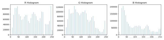
使用的图片为：

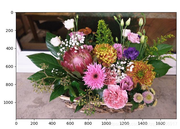
绘制HSV直方图，程序如下：

import matplotlib.image as mpimg
import matplotlib.pyplot as plt
import numpy as np
import cv2


def color_hist(img, nbins=32, bins_range=(0, 256)):
    img_hsv = cv2.cvtColor(img, cv2.COLOR_RGB2HSV)
    h_hist = np.histogram(img_hsv[:, :, 0], bins=nbins, range=bins_range)
    s_hist = np.histogram(img_hsv[:, :, 1], bins=nbins, range=bins_range)
    v_hist = np.histogram(img_hsv[:, :, 2], bins=nbins, range=bins_range)
    # 转换为浮点数，保证在下一步不进行整数除法
    hist_features = np.concatenate((h_hist[0], s_hist[0], v_hist[0])).astype(np.float64)
    # 对结果归一化，使直方图中所有bin的总和为1
    norm_features = hist_features / np.sum(hist_features)
    return norm_features


# 载入图片
image = mpimg.imread('hsv_image.jpg')
feature_vec = color_hist(image)
plt.imshow(image)

if feature_vec is not None:
    fig = plt.figure(figsize=(12, 6))
    plt.plot(feature_vec)
    plt.title('HSV Feature Vector', fontsize=30)
    plt.tick_params(axis='both', which='major', labelsize=20)
    fig.tight_layout()
    plt.show()
else:
    print('Your function is returing None..')

输出如下：

3.支持向量机SVM

支持向量机或“ SVM”只是一种特殊的受监督机器学习算法的名称，它可以将数据集的参数空间表征为离散类。

SVM通过将迭代方法应用于训练数据集来工作，其中训练集中的每个项目都由特征向量和标签来表征。在上图中，每个点仅由两个特征（A和B）表征。每个点的颜色与其标签相对应，或者与其在数据集中表示的对象类别相对应。

将SVM应用于此训练集可将/整个参数空间表征为离散的类。参数空间中类之间的划分称为“决策边界”，在这里由覆盖在数据上的彩色多边形表示。创建决策边界意味着考虑具有功能但没有标签的新对象时，可以立即将其分配给特定的类。换句话说，一旦对SVM进行了训练，就可以将其用于对象识别。

Scikit-Learn中的SVM

sklearnPython中的Scikit-Learn或软件包提供了多种SVM实现。为了达到我们的目的，我们将使用带有线性内核的基本SVM，因为它往往在分类方面做得很好，并且比更复杂的实现运行得更快，但是有必要查看sklearn.svm软件包中的其他可能性。

训练数据

在训练SVM之前，我们需要一个标记数据集。为了快速生成一些数据，我们将使用cluster_gen()功能，我们在前面定义的教训聚类市场细分。但是，现在，我们将为每个群集数据点以及x和y位置提供函数输出标签

n_clusters = 5
clusters_x, clusters_y, labels = cluster_gen(n_clusters)

在这种情况下，特征是聚类点的x和y位置，标签只是与每个聚类关联的数字。要将它们用作训练数据，需要转换为sklearn.svm.SVC（）期望的格式，它是形状(n_samples, m_features)和长度标签的功能集n_samples（在这种情况下，n_samples是聚类点的总数，m_features为2 ）。在机器学习应用程序中，通常会调用功能集X和标签y。

根据cluster_gen()的输出格式，可以创建如下特性和标签:

import numpy as np
X = np.float32((np.concatenate(clusters_x), np.concatenate(clusters_y))).transpose()
y = np.float32((np.concatenate(labels)))

整理好训练数据后，sklearn就可以轻松创建和训练SVM！

from sklearn import svm
svc = svm.SVC(kernel='linear').fit(X, y)

在下面的程序中，可以更改数据集。可以在np.random.seed(424)语句中更改数字以生成其他数据集。可以查看sklearn.svm.SVC（）的文档，以查看可以调整的参数以及结果如何变化。

import numpy as np
import matplotlib.pyplot as plt
from sklearn import svm

# 定义一个函数来生成集群
def cluster_gen(n_clusters, pts_minmax=(100, 500), x_mult=(2, 7), y_mult=(2, 7),
                             x_off=(0, 50), y_off=(0, 50)):
    # n_clusters = 要生成的集群数量
    # pts_minmax = 每个集群的点数范围
    # x_mult = 乘法器的范围，在x方向修改集群的大小
    # y_mult = 乘法器的范围，在y方向修改集群的大小
    # x_off = 簇在x方向上的位置偏移范围
    # y_off = 簇在y方向上的位置偏移范围

    # 初始化一些空列表以接收集群成员位置
    clusters_x = []
    clusters_y = []
    labels = []

    # 生成随机值给定参数范围
    n_points = np.random.randint(pts_minmax[0], pts_minmax[1], n_clusters)
    x_multipliers = np.random.randint(x_mult[0], x_mult[1], n_clusters)
    y_multipliers = np.random.randint(y_mult[0], y_mult[1], n_clusters)
    x_offsets = np.random.randint(x_off[0], x_off[1], n_clusters)
    y_offsets = np.random.randint(y_off[0], y_off[1], n_clusters)

    # 生成随机集群给定参数值
    for idx, npts in enumerate(n_points):

        xpts = np.random.randn(npts) * x_multipliers[idx] + x_offsets[idx]
        ypts = np.random.randn(npts) * y_multipliers[idx] + y_offsets[idx]
        clusters_x.append(xpts)
        clusters_y.append(ypts)
        labels.append(np.zeros_like(xpts) + idx)

    # 返回集群位置和标签
    return clusters_x, clusters_y, labels

np.random.seed(424)  # 更改编号以生成不同的集群

n_clusters = 3
clusters_x, clusters_y, labels = cluster_gen(n_clusters)

# 转换为sklearn格式的培训数据集
X = np.float32((np.concatenate(clusters_x), np.concatenate(clusters_y))).transpose()
y = np.float32((np.concatenate(labels)))

# 创建一个SVM实例，并对数据进行拟合。
ker = 'linear'
svc = svm.SVC(kernel=ker).fit(X, y)

# 创建一个网格，我们将使用彩色来确定表面
# Plotting Routine courtesy of: http://scikit-learn.org/stable/auto_examples/svm/plot_iris.html#sphx-glr-auto-examples-svm-plot-iris-py
# 注意:这种配色方案在> 7个簇或更多的地方失效

h = 0.2  # 在网格中的步长
x_min, x_max = X[:, 0].min() - 1, X[:, 0].max() + 1  # -1 and +1 to add some margins
y_min, y_max = X[:, 1].min() - 1, X[:, 1].max() + 1
xx, yy = np.meshgrid(np.arange(x_min, x_max, h),
                     np.arange(y_min, y_max, h))

# 对网格的每个块进行分类(用于分配其颜色)
Z = svc.predict(np.c_[xx.ravel(), yy.ravel()])

# 将结果放入颜色图中
Z = Z.reshape(xx.shape)
plt.contourf(xx, yy, Z, cmap=plt.cm.coolwarm, alpha=0.8)

# 绘制训练点
plt.scatter(X[:, 0], X[:, 1], c=y, cmap=plt.cm.coolwarm, edgecolors='black')
plt.xlim(xx.min(), xx.max())
plt.ylim(yy.min(), yy.max())
plt.xticks(())
plt.yticks(())
plt.title('SVC with '+ker+' kernel', fontsize=20)
plt.show()

输出如下：

4.SVM图像分类

我们在，我们已经了解了如何使用SVM对多类数据集进行分类，但是只有两个功能描述了每个元素。有了点云数据，w将拥有一个丰富的功能集，其中包含颜色和表面法线直方图。具有丰富功能集的分类与具有两个功能的分类工作相同，但更难以可视化，因此我们将通过使用颜色直方图的图像分类示例进行学习。

为了演示图像分类，我们将借鉴自动驾驶汽车纳米学位计划的一项练习。在本练习中，数据集由数百个汽车图像以及可能在汽车场景中发现的其他图像组成，但还有其他一些。我们的目标是训练SVM根据由颜色直方图组成的输入特征向量来识别图像是否包含汽车。在这里，我们将介绍一些与准备训练数据和评估分类器性能有关的概念。

首先，我们会在汽车图像和非汽车图像中为每个图像提取颜色特征，然后将特征向量缩放为零均值和单位方差。

之后，我们将定义标签向量，将数据洗牌并将其拆分为训练和测试集，最后，定义一个分类器并对其进行训练。

这种情况下，标签向量将只是一个二进制向量，指示数据集中的每个特征向量是对应于汽车还是非汽车（汽车为1，非汽车为0）。在这里，我们有一个称为extract_features()的函数，该color_hist()函数将调用在上一个练习中定义的函数，并从图像数据集中生成一系列特征。

# Define a function to extract features from a list of images
# Have this function call color_hist()
def extract_features(imgs, hist_bins=32, hist_range=(0, 256)):
    # Create a list to append feature vectors to
    features = []
    # Iterate through the list of images
    for file in imgs:
        # Read in each one by one
        image = mpimg.imread(file)
        # Apply color_hist() 
        hist_features = color_hist(image, nbins=hist_bins, bins_range=hist_range)
        # Append the new feature vector to the features list
        features.append(hist_features)
    # Return list of feature vectors
    return features

给定汽车和非汽车特征的列表，我们可以定义标签矢量（只是一堆的一和零），如下所示：

import numpy as np
# Define a labels vector based on features lists
y = np.hstack((np.ones(len(car_features)), 
              np.zeros(len(notcar_features))))
          

接下来，我们将叠加和缩放我们的特征向量。堆叠成一个单独的数组是为了得到sklearn所期望的格式。扩展是一个更微妙的问题。在堆叠的阵列中，每个要素将占据一列。当某些功能的大小远远大于其他功能时，可能会导致分类器的性能下降。因此，执行每列归一化以确保所有特征大致相同的比例（在这里，我们将平均值和单位方差缩放为零）始终是一个好方法。

from sklearn.preprocessing import StandardScaler
# Create an array stack of feature vectors
X = np.vstack((car_features, notcar_features)).astype(np.float64)
# Fit a per-column scaler
X_scaler = StandardScaler().fit(X)
# Apply the scaler to X
scaled_X = X_scaler.transform(X)

现在我们准备好将数据洗牌并将其分为训练和测试集。在单独的数据集上测试分类器总是一个好主意，但是首先应该随机处理数据。这确保了数据的任何排序(例如，数据集开头的一堆红色汽车和结尾的蓝色汽车)都不会影响分类器的训练。

为此，我们将使用Scikit-Learn train_test_split()函数，但值得注意的是，该函数最近从sklearn.cross_validation软件包（sklearn版本== 0.17）移动到sklearn.model_selection软件包（sklearn版本> = 0.18）。

在测验编辑器中，我们仍在运行sklearnv0.17，因此我们将其导入为：

from sklearn.cross_validation import train_test_split
# But, if you are using scikit-learn >= 0.18 then use this:
# from sklearn.model_selection import train_test_split

train_test_split()执行数据的随机播放和拆分，可以这样称呼它（此处选择每次使用不同的随机状态初始化随机播放）：

# Split up data into randomized training and test sets
rand_state = np.random.randint(0, 100)
X_train, X_test, y_train, y_test = train_test_split(
    scaled_X, y, test_size=0.2, random_state=rand_state)

现在，现在就可以定义和训练分类器了。在这里，我们将对线性内核使用相同的SVC。要定义和训练分类器，只需几行代码：

from sklearn.svm import LinearSVC
# Use a linear SVC (support vector classifier)
svc = SVC(kernel='linear')
# Train the SVC
svc.fit(X_train, y_train)

然后，可以像这样检查测试数据集上分类器的准确性：

print('Test Accuracy of SVC = ', svc.score(X_test, y_test))

或者，可以对测试数据的一部分进行预测，然后直接与基本事实进行比较：

print('My SVC predicts: ', svc.predict(X_test[0:10].reshape(1, -1)))
print('For labels: ', y_test[0:10])

histbin在下面的练习中使用参数值，以查看分类器准确性和训练时间如何随特征向量输入而变化。

完整程序如下：

import matplotlib.image as mpimg
import matplotlib.pyplot as plt
import numpy as np
import cv2
import glob
import time
from sklearn.svm import SVC
from sklearn.preprocessing import StandardScaler
# NOTE: the next import is only valid
# for scikit-learn version <= 0.17
# if you are using scikit-learn >= 0.18 then use this:
from sklearn.model_selection import train_test_split
# from sklearn.cross_validation import train_test_split


# 定义一个函数来计算颜色直方图特征,输入为图片，返回特征向量
def color_hist(img, nbins=32, bins_range=(0, 256)):
    # 将RGB转换为HSV
    hsv_img = cv2.cvtColor(img, cv2.COLOR_RGB2HSV)
    # 计算各个HSV通道的直方图
    h_hist = np.histogram(hsv_img[:, :, 0], bins=nbins, range=bins_range)
    s_hist = np.histogram(hsv_img[:, :, 1], bins=nbins, range=bins_range)
    v_hist = np.histogram(hsv_img[:, :, 2], bins=nbins, range=bins_range)
    # 将直方图连接成单个特征向量
    hist_features = np.concatenate((h_hist[0], s_hist[0], v_hist[0])).astype(np.float64)
    # 归一化
    norm_features = hist_features / np.sum(hist_features)
    # 返回特征向量
    return norm_features


# 定义一个从图像列表中提取特征的函数，输入为图片列表，返回特征向量列表
# 这个函数调用color_hist()
def extract_features(imgs, hist_bins=32, hist_range=(0, 256)):
    # 创建一个列表来附加特征向量
    features = []
    # 遍历图像列表
    for file in imgs:
        image = mpimg.imread(file)
        # 应用color_hist ()
        hist_features = color_hist(image, nbins=hist_bins, bins_range=hist_range)
        # 将新的特征向量附加到特征列表中
        features.append(hist_features)
    # 返回特征向量列表
    return features


# 读取汽车和非汽车图像
images = glob.glob('*/*/*/*.jpeg')
cars = []
notcars = []


for image in images:
    if 'image' in image or 'extra' in image:
        notcars.append(image)
    else:
        cars.append(image)

if cars == [] or notcars == []:
    print("images is empty! please check your images path!")

# TODO play with this value to see how your classifier
# 在不同的场景下执行
histbin = 32
# 读取汽车和非汽车图像列表，应用extract_features函数
car_features = extract_features(cars, hist_bins=histbin, hist_range=(0, 256))
notcar_features = extract_features(notcars, hist_bins=histbin, hist_range=(0, 256))

# 创建一个特征向量数组堆叠
X = np.vstack((car_features, notcar_features)).astype(np.float64)
# 确定每列的定标器
X_scaler = StandardScaler().fit(X)
# 把定标器应用到X轴上
scaled_X = X_scaler.transform(X)

# 定义标签向量
y = np.hstack((np.ones(len(car_features)), np.zeros(len(notcar_features))))

# 将数据分成随机的训练和测试集
rand_state = np.random.randint(0, 100)
X_train, X_test, y_train, y_test = train_test_split(
    scaled_X, y, test_size=0.2, random_state=rand_state)

print('Dataset includes', len(cars), 'cars and', len(notcars), 'not-cars')
print('Using', histbin, 'histogram bins')
print('Feature vector length:', len(X_train[0]))
# 使用线性SVC
svc = SVC(kernel='linear')
# SVC的训练时间
t = time.time()
svc.fit(X_train, y_train)
t2 = time.time()
print(round(t2-t, 2), 'Seconds to train SVC...')
# SVC的分数
print('Test Accuracy of SVC = ', round(svc.score(X_test, y_test), 4))
# 单个样本的预测时间
t = time.time()
n_predict = 10
print('My SVC predicts: ', svc.predict(X_test[0:n_predict]))
print('For these', n_predict, 'labels: ', y_test[0:n_predict])
t2 = time.time()
print(round(t2-t, 5), 'Seconds to predict', n_predict,'labels with SVC')

程序输出为：

Dataset includes 1196 cars and 1125 not-cars
Using 32 histogram bins
Feature vector length: 96
0.07 Seconds to train SVC...
Test Accuracy of SVC =  0.9914
My SVC predicts:  [1. 1. 1. 1. 1. 0. 1. 0. 0. 0.]
For these 10 labels:  [1. 1. 1. 1. 1. 0. 1. 0. 0. 0.]
0.00099 Seconds to predict 10 labels with SVC

5.识别实例

这个练习提供了一个非常简单的gazebo世界，我们可以从练习1和练习2中从点云中分割的对象中提取颜色和形状特征，以便训练分类器来检测它们。

本练习的目标是训练SVM识别场景中的特定对象。为此，首先要提取一组特征和标签，然后训练SVM分类器，最后使用分类器预测分节点云中的对象。

如果已经克隆了robond感知练习库，那么需要做的就是再次获取git pull以获得练习3的代码。

ps:这个练习需要ROS，所以需要在Udacity提供的VM中或在自己的本地Linux/ROS安装上完成这些步骤。

环境配置

如果完成了练习1和练习2，那么在~/catkin_ws/src目录中已经有一个sensor_stick文件夹了。应该首先复制为练习cp2编写的Python脚本(segmentation .py)，然后将旧的sensor_stick文件夹替换为存储库中包含在练习3目录中的新sensor_stick文件夹。

如果还没有sensor_stick目录，那么首先复制/移动sensor_stick文件夹到活动ros工作区的~/catkin_ws/src目录。

从练习3目录:

cp -r sensor_stick/ ~/catkin_ws/src/

通过使用该rosdep install工具并运行，确保已解决所有依赖项

catkin_make：
$ cd ~/catkin_ws
$ rosdep install --from-paths src --ignore-src --rosdistro=kinetic -y
$ catkin_make

如果它们还不在其中，将以下行添加到.bashrc文件中

$ export GAZEBO_MODEL_PATH=~/catkin_ws/src/sensor_stick/models
$ source ~/catkin_ws/devel/setup.bash

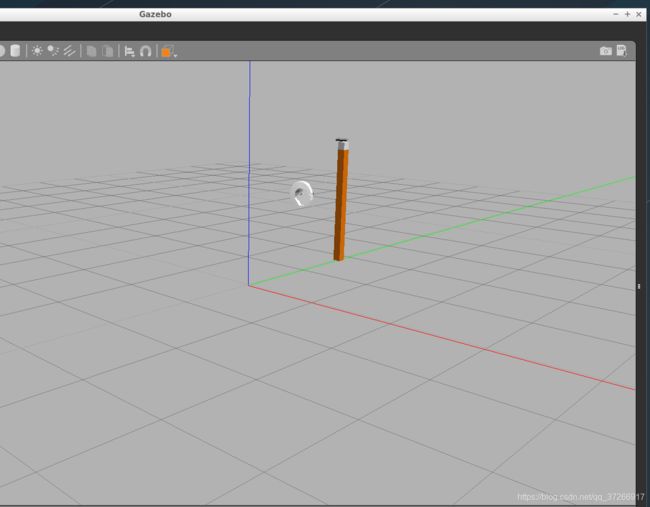
产生特征

要开始生成功能，启动training.launch文件以启动Gazebo环境。一个空的环境应该只在场景中出现带RGBD相机的棒状结构：

$ cd ~/catkin_ws
$ roslaunch sensor_stick training.launch

注意终端中的错误，如果凉亭崩溃或没有出现，再可以尝试一次，有时需要尝试几次。

ps:看来之前的出错的原因有可能和程序本身的bug有关系

捕捉功能

接下来，打开一个新的终端，运行capture_features.py脚本以捕获并保存环境中每个对象的功能。该脚本以随机方向生成每个对象（每个对象默认5个方向），并根据每个随机方向产生的点云计算特征。

$ cd ~/catkin_ws
$ rosrun sensor_stick capture_features.py

可以看到对象正在在Gazebo生成。每个随机方向需要5-10秒(取决于机器的资源)。总共有7个对象，所以需要一段时间才能完成。当它运行结束时，应该有一个包含数据集的特性和标签的 training_set.sav 文件。
注意: training_set.sav 文件将保存在的catkin_ws文件夹中。

训练SVM

一旦特征提取成功完成，就可以训练模型了。

$ rosrun sensor_stick train_svm.py

运行此命令后，将在终端上获得一些有关分类器总体准确性的文本输出，并且将弹出两个图，显示分类器对各种对象的相对准确性：

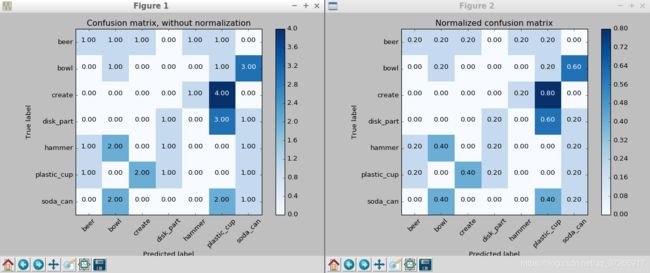
这些图显示了分类器的两个不同版本的混淆矩阵。左边是原始计数，右边是占总数的百分比。假设在特征生成过程中以随机方向生成对象，所以每次生成的图都不一样。

运行上面的命令还将导致训练的模型保存在model.sav文件中。

注意：此model.sav文件将保存在catkin_ws文件夹中。

改善模型

我们的混淆矩阵生成的非常不理想。是因为还没有真正生成有意义的特性。要获得更好的特性，在/sensor_stick/src/sensor_stick/中打开features.py脚本(这可能看起来像一个奇怪的目录结构，但这是设置内部Python包的首选ROS方法)。在这个脚本中，有两个名为compute_color_histograms()和compute_normal_histograms()的函数。

在compute_color_histograms()和compute_normal_histograms()函数中，有从点云中提取的三个值列表，其中channel_*_vals(表示颜色)和norm_*_vals(表示法线)。可以使用之前提到的直方图技术来存储这些数据。在加入直方图之后，将它们连接到一个特征向量中并进行标准化，以创建函数输出(normed_features)。再次运行capture_features.py，train_svm.py查看效果。

features.py函数如下所示：

import matplotlib.colors
import matplotlib.pyplot as plt
import numpy as np
from pcl_helper import *


def rgb_to_hsv(rgb_list):
    rgb_normalized = [1.0*rgb_list[0]/255, 1.0*rgb_list[1]/255, 1.0*rgb_list[2]/255]
    hsv_normalized = matplotlib.colors.rgb_to_hsv([[rgb_normalized]])[0][0]
    return hsv_normalized


def compute_color_histograms(cloud, using_hsv=False):

    # Compute histograms for the clusters
    point_colors_list = []

    # Step through each point in the point cloud
    for point in pc2.read_points(cloud, skip_nans=True):
        rgb_list = float_to_rgb(point[3])
        if using_hsv:
            point_colors_list.append(rgb_to_hsv(rgb_list) * 255)
        else:
            point_colors_list.append(rgb_list)

    # Populate lists with color values
    channel_1_vals = []
    channel_2_vals = []
    channel_3_vals = []

    for color in point_colors_list:
        channel_1_vals.append(color[0])
        channel_2_vals.append(color[1])
        channel_3_vals.append(color[2])
    
    # TODO: Compute histograms
    channel_1_hist = np.histogram(channel_1_vals, bins=32, range=(0, 256))
    channel_2_hist = np.histogram(channel_2_vals, bins=32, range=(0, 256))
    channel_3_hist = np.histogram(channel_3_vals, bins=32, range=(0, 256))
    hist_features = np.concatenate((channel_1_hist[0], channel_2_hist[0], channel_3_hist[0])).astype(np.float64)
    # TODO: Concatenate and normalize the histograms
    normed_features = hist_features / np.sum(hist_features)
    return normed_features 


def compute_normal_histograms(normal_cloud):
    norm_x_vals = []
    norm_y_vals = []
    norm_z_vals = []

    for norm_component in pc2.read_points(normal_cloud,
                                          field_names = ('normal_x', 'normal_y', 'normal_z'),
                                          skip_nans=True):
        norm_x_vals.append(norm_component[0])
        norm_y_vals.append(norm_component[1])
        norm_z_vals.append(norm_component[2])

    # TODO: Compute histograms of normal values (just like with color)
    channel_1_hist = np.histogram(norm_x_vals, bins=32, range=(0, 256))
    channel_2_hist = np.histogram(norm_y_vals, bins=32, range=(0, 256))
    channel_3_hist = np.histogram(norm_z_vals, bins=32, range=(0, 256))
    hist_features = np.concatenate((channel_1_hist[0], channel_2_hist[0], channel_3_hist[0])).astype(np.float64)
    # TODO: Concatenate and normalize the histograms
    normed_features = hist_features / np.sum(hist_features)

    return normed_features

create_features.py如下所示

#!/usr/bin/env python
import numpy as np
import pickle
import rospy

from sensor_stick.pcl_helper import *
from sensor_stick.training_helper import spawn_model
from sensor_stick.training_helper import delete_model
from sensor_stick.training_helper import initial_setup
from sensor_stick.training_helper import capture_sample
from sensor_stick.features import compute_color_histograms
from sensor_stick.features import compute_normal_histograms
from sensor_stick.srv import GetNormals
from geometry_msgs.msg import Pose
from sensor_msgs.msg import PointCloud2


def get_normals(cloud):
    get_normals_prox = rospy.ServiceProxy('/feature_extractor/get_normals', GetNormals)
    return get_normals_prox(cloud).cluster


if __name__ == '__main__':
    rospy.init_node('capture_node')

    models = [\
       'beer',
       'bowl',
       'create',
       'disk_part',
       'hammer',
       'plastic_cup',
       'soda_can']

    # Disable gravity and delete the ground plane
    initial_setup()
    labeled_features = []

    for model_name in models:
        spawn_model(model_name)

        for i in range(10):
            # make five attempts to get a valid a point cloud then give up
            sample_was_good = False
            try_count = 0
            while not sample_was_good and try_count < 5:
                sample_cloud = capture_sample()
                sample_cloud_arr = ros_to_pcl(sample_cloud).to_array()

                # Check for invalid clouds.
                if sample_cloud_arr.shape[0] == 0:
                    print('Invalid cloud detected')
                    try_count += 1
                else:
                    sample_was_good = True

            # Extract histogram features
            chists = compute_color_histograms(sample_cloud, using_hsv=True)
            normals = get_normals(sample_cloud)
            nhists = compute_normal_histograms(normals)
            feature = np.concatenate((chists, nhists))
            labeled_features.append([feature, model_name])

        delete_model()


    pickle.dump(labeled_features, open('training_set.sav', 'wb'))

再次运行train_svm.py，得到的输出如下，可以看到，得到的混淆矩阵和结果好了很多。

要修改每个对象随机派生的次数，在capture_features.py中查找以range(5)中的for i in range(5)的for循环。增加此值以增加为每个对象捕获特性的次数。

使用HSV，在capture_features.py中找到调用compute_color_histograms()的行，并将标志更改为using_hsv=True。

SVM训练过程，在train_svm.py中：

#!/usr/bin/env python
import pickle
import itertools
import numpy as np
import matplotlib.pyplot as plt
from sklearn import svm
from sklearn.preprocessing import LabelEncoder, StandardScaler
from sklearn import cross_validation
from sklearn import metrics

def plot_confusion_matrix(cm, classes,
                          normalize=False,
                          title='Confusion matrix',
                          cmap=plt.cm.Blues):
    """
    This function prints and plots the confusion matrix.
    Normalization can be applied by setting `normalize=True`.
    """
    if normalize:
        cm = cm.astype('float') / cm.sum(axis=1)[:, np.newaxis]
    plt.imshow(cm, interpolation='nearest', cmap=cmap)
    plt.title(title)
    plt.colorbar()
    tick_marks = np.arange(len(classes))
    plt.xticks(tick_marks, classes, rotation=45)
    plt.yticks(tick_marks, classes)

    thresh = cm.max() / 2.
    for i, j in itertools.product(range(cm.shape[0]), range(cm.shape[1])):
        plt.text(j, i, '{0:.2f}'.format(cm[i, j]),
                 horizontalalignment="center",
                 color="white" if cm[i, j] > thresh else "black")

    plt.tight_layout()
    plt.ylabel('True label')
    plt.xlabel('Predicted label')

# 从磁盘加载培训数据
training_set = pickle.load(open('training_set.sav', 'rb'))

# 将特性和标签格式化，以便与scikit learn一起使用
feature_list = []
label_list = []

for item in training_set:
    if np.isnan(item[0]).sum() < 1:
        feature_list.append(item[0])
        label_list.append(item[1])

print('Features in Training Set: {}'.format(len(training_set)))
print('Invalid Features in Training set: {}'.format(len(training_set)-len(feature_list)))

X = np.array(feature_list)
# Fit a per-column scaler
X_scaler = StandardScaler().fit(X)
# Apply the scaler to X
X_train = X_scaler.transform(X)
y_train = np.array(label_list)

# 将标签字符串转换为数字编码
encoder = LabelEncoder()
y_train = encoder.fit_transform(y_train)

# 创建分类器
clf = svm.SVC(kernel='linear')

# 建立5倍交叉验证
kf = cross_validation.KFold(len(X_train),
                            n_folds=5,
                            shuffle=True,
                            random_state=1)

# 进行交叉验证
scores = cross_validation.cross_val_score(cv=kf,
                                         estimator=clf,
                                         X=X_train,
                                         y=y_train,
                                         scoring='accuracy'
                                        )
print('Scores: ' + str(scores))
print('Accuracy: %0.2f (+/- %0.2f)' % (scores.mean(), 2*scores.std()))

# 收集预测
predictions = cross_validation.cross_val_predict(cv=kf,
                                          estimator=clf,
                                          X=X_train,
                                          y=y_train
                                         )

accuracy_score = metrics.accuracy_score(y_train, predictions)
print('accuracy score: '+str(accuracy_score))

confusion_matrix = metrics.confusion_matrix(y_train, predictions)

class_names = encoder.classes_.tolist()


# 训练分类器
clf.fit(X=X_train, y=y_train)

model = {'classifier': clf, 'classes': encoder.classes_, 'scaler': X_scaler}

# 将分类器保存到磁盘
pickle.dump(model, open('model.sav', 'wb'))

# 绘制非标准化混淆矩阵
plt.figure()
plot_confusion_matrix(confusion_matrix, classes=encoder.classes_,
                      title='Confusion matrix, without normalization')

# 绘制归一化混淆矩阵
plt.figure()
plot_confusion_matrix(confusion_matrix, classes=encoder.classes_, normalize=True,
                      title='Normalized confusion matrix')

plt.show()

来看一下model.sav文件中的信息：

{
'classes'	:	array(['beer', 'bowl', 'create', 'disk_part', 'hammer', 'plastic_cup','soda_can'], dtype='|S11'), 
'classifier':	SVC(C=1.0, cache_size=200, class_weight=None, coef0=0.0,
				decision_function_shape='ovr', degree=3, gamma='auto', kernel='linear',
				max_iter=-1, probability=False, random_state=None, shrinking=True,
				tol=0.001, verbose=False), 
'scaler'	:	StandardScaler(copy=True, with_mean=True, with_std=True)
}

物体识别

首先，必须构建节点来分割点云。

复制sensor_stick/scripts/目录中的template.py文件，并将其命名为类似object_recognition.py的名称。

首先，创建一些要接收的空列表

    # Classify the clusters!
    detected_objects_labels = []
    detected_objects = []

接下来，编写一个for循环来遍历每个分段的集群。

	# 遍历各个集群，以索引和点的列表
    for index, pts_list in enumerate(cluster_indices):
        # 使用之前练习的程序
        pcl_cluster = cloud_objects.extract(pts_list)
        # TODO: convert the cluster from pcl to ROS using helper function
        cloud_cluster = pcl_to_ros(pcl_cluster)
        # 提取直方图特征
        # TODO: complete this step just as is covered in capture_features.py
        # 获取色彩（color）直方图
	    chists = compute_color_histograms(cloud_cluster, using_hsv=True)
        # 计算法线（normal）的直方图
	    normals = get_normals(cloud_cluster)
        nhists = compute_normal_histograms(normals)
        # 将色彩和法线直方图联结作为特征
        feature = np.concatenate((chists, nhists))
        # 预测
        prediction = clf.predict(scaler.transform(feature.reshape(1,-1)))
        # 标签从数字转换为字符
        label = encoder.inverse_transform(prediction)[0]
        detected_objects_labels.append(label)

        # 定义标签位置，将标签发布到RViz
        label_pos = list(white_cloud[pts_list[0]])
        label_pos[2] += .4
        object_markers_pub.publish(make_label(label,label_pos, index))

        # 将检测到的对象添加到检测到的对象列表中。
        do = DetectedObject()
        do.label = label
        do.cloud = cloud_cluster
        detected_objects.append(do)

    rospy.loginfo('Detected {} objects: {}'.format(len(detected_objects_labels), detected_objects_labels))

    # Publish the list of detected objects
    detected_objects_pub.publish(detected_objects)

下面，在if……name__ == '……main__'开头的部分，添加以下代码来创建一些新的发布者，并加载训练完成的模型中:

	# create two publishers
    object_markers_pub = rospy.Publisher('/object_markers', Marker, queue_size=1)
    detected_objects_pub = rospy.Publisher('detecter_objects', DetectedObjectsArray, queue_size=1)
    # 加载模型
    model = pickle.load(open('model.sav', 'rb'))
    clf = model['classifier']
    # 用0和n_classes-1之间的值对标签进行编码。
    encoder = LabelEncoder()
    encoder.classes_ = model['classes']
    # 定标器
    scaler = model['scaler']

完整程序如下,在ros中不要使用中文注释：

#!/usr/bin/env python

import numpy as np
import sklearn
from sklearn.preprocessing import LabelEncoder

import pickle

from sensor_stick.srv import GetNormals
from sensor_stick.features import compute_color_histograms
from sensor_stick.features import compute_normal_histograms
from visualization_msgs.msg import Marker

from sensor_stick.marker_tools import *
from sensor_stick.msg import DetectedObjectsArray
from sensor_stick.msg import DetectedObject
from sensor_stick.pcl_helper import *

# 定义获取点云法线的函数
def get_normals(cloud):
    get_normals_prox = rospy.ServiceProxy('/feature_extractor/get_normals', GetNormals)
    return get_normals_prox(cloud).cluster


# Callback function for your Point Cloud Subscriber
def pcl_callback(pcl_msg):
    # TODO: Convert ROS msg to PCL data
    cloud = ros_to_pcl(pcl_msg)
    # TODO: Voxel Grid Downsampling
    vox = cloud.make_voxel_grid_filter()
    LEAF_SIZE = 0.02
    vox.set_leaf_size(LEAF_SIZE, LEAF_SIZE, LEAF_SIZE)
    cloud = vox.filter()
    # TODO: PassThrough Filter
    passthrough = cloud.make_passthrough_filter()
    filter_axis = 'z'
    passthrough.set_filter_field_name(filter_axis)
    axis_min = 0.76
    axis_max = 1.3
    passthrough.set_filter_limits(axis_min, axis_max)
    cloud = passthrough.filter()
    # TODO: RANSAC Plane Segmentation
    seg = cloud.make_segmenter()
    seg.set_model_type(pcl.SACMODEL_PLANE)
    seg.set_method_type(pcl.SAC_RANSAC)
    max_distance = 0.01
    seg.set_distance_threshold(max_distance)
    inlier, coefficients = seg.segment()
    # TODO: Extract inliers and outliers
    cloud_table = cloud.extract(inlier, negative=False)
    cloud_objects = cloud.extract(inlier, negative=True)
    # TODO: Euclidean Clustering
    white_cloud = XYZRGB_to_XYZ(cloud_objects)
    tree = white_cloud.make_kdtree()
    ec = white_cloud.make_EuclideanClusterExtraction()
    ec.set_ClusterTolerance(0.05)
    ec.set_MinClusterSize(10)
    ec.set_MaxClusterSize(500)
    ec.set_SearchMethod(tree)
    cluster_indices = ec.Extract()

    # 分类集群(loop through each detected cluster one at a time)
    # 初始化目标数组和标签数组
    detected_objects_labels = []
    detected_objects = []
    # 遍历各个集群，以索引和点的列表
    for index, pts_list in enumerate(cluster_indices):
        # 使用之前练习的程序
        pcl_cluster = cloud_objects.extract(pts_list)
        # TODO: convert the cluster from pcl to ROS using helper function
        cloud_cluster = pcl_to_ros(pcl_cluster)
        # 提取直方图特征
        # TODO: complete this step just as is covered in capture_features.py
        # 获取色彩（color）直方图
	    chists = compute_color_histograms(cloud_cluster, using_hsv=True)
        # 计算法线（normal）的直方图
	    normals = get_normals(cloud_cluster)
        nhists = compute_normal_histograms(normals)
        # 将色彩和法线直方图联结作为特征
        feature = np.concatenate((chists, nhists))
        # 预测
        prediction = clf.predict(scaler.transform(feature.reshape(1,-1)))
        # 标签从数字转换为字符
        label = encoder.inverse_transform(prediction)[0]
        detected_objects_labels.append(label)

        # 定义标签位置，将标签发布到RViz
        label_pos = list(white_cloud[pts_list[0]])
        label_pos[2] += .4
        object_markers_pub.publish(make_label(label,label_pos, index))

        # 将检测到的对象添加到检测到的对象列表中。
        do = DetectedObject()
        do.label = label
        do.cloud = cloud_cluster
        detected_objects.append(do)

    rospy.loginfo('Detected {} objects: {}'.format(len(detected_objects_labels), detected_objects_labels))

    # Publish the list of detected objects
    detected_objects_pub.publish(detected_objects)



if __name__ == '__main__':

    # ROS node initialization
    rospy.init_node('clustering', anonymous=True)
    # Create Subscribers
    pcl_pub = rospy.Subscriber('/sensor_stick/point_cloud', pc2.PointCloud2, pcl_callback, queue_size=1)
    # create two publishers
    object_markers_pub = rospy.Publisher('/object_markers', Marker, queue_size=1)
    detected_objects_pub = rospy.Publisher('detecter_objects', DetectedObjectsArray, queue_size=1)
    # 加载模型
    model = pickle.load(open('model.sav', 'rb'))
    clf = model['classifier']
    # 用0和n_classes-1之间的值对标签进行编码。
    encoder = LabelEncoder()
    encoder.classes_ = model['classes']
    # 定标器
    scaler = model['scaler']

    # 初始化color_list
    get_color_list.color_list = []

    # TODO: Spin while node is not shutdown
    while not rospy.is_shutdown():
        rospy.spin()

然后新开启一个终端,按原来的操作，进行如下命令

$ roslaunch sensor_stick robot_spawn.launch

在另一个终端中，运行对象识别节点（model.sav文件必须与运行此文件的目录位于同一目录中）：

$ chmod +x object_recognition.py
$ ./object_recognition.py

输出结果如下：

还是有两个模型不知道加载到哪里去了，但是剩下的几个模型还是很成功的判断出来了。