机器学习实践(2.2)LightGBM回归任务

前言

LightGBM也属于Boosting集成学习模型(还有前面文章的XGBoost)，LightGBM和XGBoost同为机器学习的集大成者。相比越来越流行的深度神经网络，LightGBM和XGBoost能更好的处理表格数据，并具有更强的可解释性，还具有易于调参、输入数据不变性等优势。

机器学习实践(1.2)XGBoost回归任务

机器学习实践(2.1)LightGBM分类任务

❤️ 本文完整脚本点此链接百度网盘链接获取 ❤️

一.轻松实现回归任务

1.1导入第三方库、数据集

"""第三方库导入"""
from lightgbm import LGBMRegressor
from sklearn import datasets
from sklearn.model_selection import train_test_split, GridSearchCV
from sklearn.metrics import r2_score, mean_squared_error
import lightgbm as lgb

"""波士顿房价数据集导入"""
data = datasets.load_boston()
# print(data)

"""训练集 验证集构建"""
X_train, X_test, y_train, y_test = train_test_split(data.data, data.target, test_size=0.2,
                                                    random_state=42)

sklearn的波士顿房价数据集共506个数据样本，8:2切分后，训练集404个数据样本，验证集102个数据样本。数据集中包括 样本特征data（13个特征）、特征名称feature_names、样本标签target（MEDV）、以及数据集位置filename（~~~\anaconda\lib\site-packages\sklearn\datasets\data\boston_house_prices.csv）

特征名称和标签解释如下：

- CRIM     per capita crime rate by town\n      # 按城镇划分的犯罪率  
- ZN       proportion of residential land zoned for lots over 25,000 sq.ft.\n  # 划分为25000平方英尺以上地块的住宅用地比例        
- INDUS    proportion of non-retail business acres per town\n     # 每每个城镇的非零售商业用地比例
- CHAS     Charles River dummy variable (= 1 if tract bounds river; 0 otherwise)\n        # 靠近查尔斯河，则为1；否则为0
- NOX      nitric oxides concentration (parts per 10 million)\n      # 一氧化氮浓度（百万分之一）
- RM       average number of rooms per dwelling\n  # 每个住宅的平均房间数      
- AGE      proportion of owner-occupied units built prior to 1940\n     # 1940年之前建造的自住单位比例  
- DIS      weighted distances to five Boston employment centres\n     # 到波士顿五个就业中心的加权距离
- RAD      index of accessibility to radial highways\n    # 辐射状公路可达性指数    
- TAX      full-value property-tax rate per $10,000\n   # 每10000美元的全额财产税税率
- PTRATIO  pupil-teacher ratio by town\n    # 按城镇划分的师生比例    
- B        1000(Bk - 0.63)^2 where Bk is the proportion of blacks by town\n  # 1000（Bk-0.63）^2其中Bk是按城镇划分的黑人比例       
- LSTAT    % lower status of the population\n    # 人口密度   
- MEDV     Median value of owner-occupied homes in $1000's\n # 住房屋的中值（单位：1000美元）

1.2模型训练

"""模型训练"""
model = LGBMRegressor()

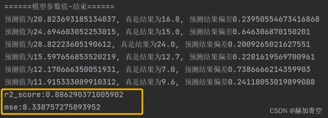
# r2_score:0.886290371005902
# mse:8.338757275893952

# 给定参数
# model = LGBMRegressor(boosting='gbdt',  # gbdt \ dart
#                       n_estimators=300,  # 迭代次数
#                       learning_rate=0.1,  # 步长
#                       max_depth=10,  # 树的最大深度
#                       seed=42,  # 指定随机种子，为了复现结果
#                       )

# r2_score:0.9043019057586194
# mse:7.017903291953562

model.fit(X_train, y_train)

LGBMRegressor()是没有指定参数，模型使用默认参数如下。也可以指定参数例如指定boosting='dart'等。训练的模型参数如下：

parameters:
[boosting: gbdt]
[objective: regression]
[metric: l2]
[tree_learner: serial]
[device_type: cpu]
[data: ]
[valid: ]
[num_iterations: 100]
[learning_rate: 0.1]
[num_leaves: 31]
[num_threads: -1]
[deterministic: 0]
[force_col_wise: 0]
[force_row_wise: 0]
[histogram_pool_size: -1]
[max_depth: -1]
......

1.3模型验证

模型效果的验证，简单直接的可以通过验证集来实现。实际项目中通常将整个数据集按照7:3:1比例划分为训练集、验证集、测试集。本例使用验证集验证模型准确性。
回归任务的评估指标只要有 r2_score 和 mse，其中 r2_score 越趋近于1越好，mse 越小越好。
R2 = 1 - (SSE / TSS)，其中，SSE(sum of squared errors )是模型预测值与实际观测值之间差异的平方和，TSS(total sum of squares)是所有观测值与其均值差异的平方和。

y_pred = model.predict(X_test)
# print(y_pred)

for m, n in zip(y_pred, y_test):
    if m / n - 1 > 0.2:
        print('预测值为{0}, 真是结果为{1}, 预测结果偏差大于20%'.format(m, n))


def metrics_sklearn(y_valid, y_pred_):
    """模型效果评估"""
    r2 = r2_score(y_valid, y_pred_)
    print('r2_score:{0}'.format(r2))

    mse = mean_squared_error(y_valid, y_pred_)
    print('mse:{0}'.format(mse))


"""模型效果评估"""
metrics_sklearn(y_test, y_pred)

结果中仅打印了预测误差在20%以上的预测数据。

二.模型调参

def adj_params():
    """模型调参"""
    params = {
        'n_estimators': [100, 200, 300, 400],
        # 'learning_rate': [0.01, 0.03, 0.05, 0.1],
        'max_depth': [5, 8, 10, 12]
    }

    other_params = {'learning_rate': 0.1, 'seed': 42}
    model_adj = LGBMRegressor(**other_params)

    # sklearn提供的调参工具，训练集k折交叉验证(消除数据切分产生数据分布不均匀的影响)
    optimized_param = GridSearchCV(estimator=model_adj, param_grid=params, scoring='r2', cv=5, verbose=1)
    # 模型训练
    optimized_param.fit(X_train, y_train)

    # 对应参数的k折交叉验证平均得分
    means = optimized_param.cv_results_['mean_test_score']
    params = optimized_param.cv_results_['params']
    for mean, param in zip(means, params):
        print("mean_score: %f,  params: %r" % (mean, param))
    # 最佳模型参数
    print('参数的最佳取值：{0}'.format(optimized_param.best_params_))
    # 最佳参数模型得分
    print('最佳模型得分:{0}'.format(optimized_param.best_score_))


adj_params()

2.1网格搜索调参

params = {
        'n_estimators': [100, 200, 300, 400],
        # 'learning_rate': [0.01, 0.03, 0.05, 0.1],
        'max_depth': [5, 8, 10, 12]
    }

other_params = {'learning_rate': 0.1, 'seed': 42}

调参内容不是很多时，例如本次调参训练80次，两个参数值可以一起调整，结果如下图：

调参是个无穷无尽的过程，适可而止，切误沉溺其中本末倒置，真正决定模型效果上限的还是数据质量

2.2调参结果入模

model = LGBMRegressor(boosting='gbdt',  # gbdt \ dart
                      n_estimators=200,  # 迭代次数
                      learning_rate=0.1,  # 步长
                      max_depth=5,  # 树的最大深度
                      seed=42,  # 指定随机种子，为了复现结果
                      )

model.fit(X_train, y_train)

基础模型boosting='gbdt'，最大深度max_depth=5， 迭代次数n_estimators=200 参数入模，fit()训练带参的模型，模型的参数和评估见下方（三.模型保存、加载、调用预测）

三.模型保存、加载、调用预测

3.1模型保存、加载、调用预测

"""模型保存"""
model.booster_.save_model('lgb_regressor_boston.txt')

"""模型加载"""
rgs = lgb.Booster(model_file='lgb_regressor_boston.txt')

"""模型参数打印"""
print('模型参数值-开始'.center(20, '='))
# lightgbm模型参数直接打开模型文件查看更为方便
model_params = rgs.dump_model()
print(model_params)
print('模型参数值-结束'.center(20, '='))

"""预测验证数据"""
y_pred = rgs.predict(X_test)

"""模型效果评估"""
metrics_sklearn(y_test, y_pred)

模型参数打印和预测评估结果如图，不再赘述。

3.2模型参数

经过上面脚本’lgb_regressor_boston.txt’是已经保存到本地的模型文件，可以打开文件查看参数，其中
最开始是 树tree 的信息；

tree
version=v3
num_class=1
num_tree_per_iteration=1
label_index=0
max_feature_idx=12
objective=regression
feature_names=Column_0 Column_1 Column_2 Column_3 Column_4 Column_5 Column_6 Column_7 Column_8 Column_9 Column_10 Column_11 Column_12
feature_infos=[

每个tree信息都会存在，trees之后是feature_importances特征重要性信息，几乎在文件末尾；

......
end of trees

feature_importances:
Column_12=289
Column_7=237
Column_5=230
Column_6=174
Column_0=155
Column_11=140
Column_4=138
Column_9=97
Column_10=68
Column_2=38
Column_3=34
Column_1=21
Column_8=16

结尾是 parameters 参数和 pandas_categorical pandas经过虚拟化的类别信息。

parameters:
[boosting: gbdt]
[objective: regression]
[metric: l2]
[tree_learner: serial]
[device_type: cpu]
[data: ]
[valid: ]
[num_iterations: 200]
[learning_rate: 0.1]
[num_leaves: 31]
[num_threads: -1]
[deterministic: 0]
[force_col_wise: 0]
[force_row_wise: 0]
[histogram_pool_size: -1]
[max_depth: 5]
[min_data_in_leaf: 20]
......

end of parameters

pandas_categorical:null

---

附加——深入学习XGBoost

附加1.模型调参、训练、保存、评估和预测

见《XGBoost模型调参、训练、评估、保存和预测》 ，包含模型脚本文件

附加2.算法原理

见《XGBoost算法原理及基础知识》 ，包括集成学习方法，XGBoost模型、目标函数、算法，公式推导等

附加3.分类任务的评估指标值详解

见《分类任务评估1——推导sklearn分类任务评估指标》，其中包含了详细的推理过程；
见《分类任务评估2——推导ROC曲线、P-R曲线和K-S曲线》，其中包含ROC曲线、P-R曲线和K-S曲线的推导与绘制；

附加4.模型中树的绘制和模型理解

见《Graphviz绘制模型树1——软件配置与XGBoost树的绘制》，包含Graphviz软件的安装和配置，以及to_graphviz()和plot_trees()两个画图函数的部分使用细节；
见《Graphviz绘制模型树2——XGBoost模型的可解释性》，从模型中的树着手解释XGBoost模型，并用EXCEL构建出模型。

附加5.XGBoost实践

见机器学习实践(1.1)XGBoost分类任务，包含二分类、多分类任务以及多分类的评估方法。
见机器学习实践(1.2)XGBoost回归任务，包含回归任务模型训练、评估（R2、MSE）
见机器学习实践(2.1)LightGBM分类任务，包含LightGBM二分类、多分类任务及评估方法。

❤️ 机器学习内容持续更新中… ❤️

---

声明：本文所载信息不保证准确性和完整性。文中所述内容和意见仅供参考，不构成实际商业建议，可收藏可转发但请勿转载，如有雷同纯属巧合。