电路综合-基于简化实频的集总参数电路匹配3-将任意阻抗用集总参数匹配至归一化阻抗

电路综合-基于简化实频的集总参数电路匹配3-将任意阻抗用集总参数匹配至归一化阻抗

前面的相关理论：
电路综合-基于简化实频的集总参数电路匹配1
电路综合-基于简化实频的集总参数电路匹配2-得出解析解并综合
理论这两个已经介绍过了，直接给出案例

代码链接：https://download.csdn.net/download/weixin_44584198/88547435

1、案例

目标：将30+j50的阻抗在0.8-1MHz内匹配至50欧姆
代码：

clear
clc
close all

%% 分析的计算点数   越多越精密
Z0=50;
% 理想增益设定为1
T0=1;
% 使用阻抗函数进行综合
KFlag=1;
% sign为+-1，结构不同
sign=1;



% Step 1: Generate the load data
freq_arrary=[0.8 0.9 1]*1e6;
WBR=freq_arrary/max(freq_arrary);
RLA=[30 30 30]/Z0;
XLA=[50 50 50]/Z0;

WBR2=[min(WBR):0.02:max(WBR)];
RLA=interp1(WBR,RLA,WBR2,'spline');
XLA=interp1(WBR,XLA,WBR2,'spline');
WBR=WBR2;

% Step 2: 计算出RB0的初始值
RB0=RLA*((2-T0)+2*sign*sqrt(1-T0))/T0;
XB0=Hilbert_Transform(WBR,RB0);

% Step 3: 进行优化
% Define unknowns for the optimization:
for j=1:length(RB0)
   x0(j)=(RB0(j));%Initial  
end
OPTIONS=optimset('MaxFunEvals',20000,'MaxIter',50000);
x=lsqnonlin('error_RFLT2',x0,[],[],OPTIONS,WBR,T0,RLA,XLA);
% Generate optimized driving point impedance
RBA=x;
XBA=Hilbert_Transform(WBR,RBA);

% 画图参数
RTSQ=(RB0+RLA).*(RB0+RLA);
XTSQ=(XB0+XLA).*(XB0+XLA);
TPG0=4*RLA.*RB0./(RTSQ+XTSQ);

RTSQ=(RBA+RLA).*(RBA+RLA);
XTSQ=(XBA+XLA).*(XBA+XLA);
TPG=4*RLA.*RBA./(RTSQ+XTSQ);



%% 下面进行解析形式的拟合与电路综合
% 确定电路元器件
Cir_num=5;
ndc=0;
W=0;
a0=1;
% 无变压器结构，终端归一化电阻
ntr=0;

% Step 4: 通过优化得出a，b的解析式
% c0=200*rand(1,Cir_num)-100;
% c0 =[156.55 -9.1399 -244.66 34.512 111.71 -21.195 -15.654];
c0=ones(1,Cir_num);
if ntr==1; x0=[c0 a0];Nx=length(x0);end;%Yes transformer case
if ntr==0; x0=c0;Nx=length(x0);end;%No transformer case
% Call optimization function lsqnonlin:    
[x,resnorm]=lsqnonlin('direct',x0,[],[],OPTIONS,ntr,ndc,W,a0,WBR,RBA,XBA);
if ntr==1; %Yes transformer case 
    for i=1:Nx-1; 
    c(i)=x(i);
    end;
    a0=x(Nx);
end
if ntr==0;% No Transformer case
    for i=1:Nx; 
        c(i)=x(i);
    end;
end
C=[c 1];
BB=Poly_Positive(C);% This positive polynomial is in w-domain
B=polarity(BB);% Now, it is transferred to p-domain        
% Generate A(-p^2) of R(-p^2)=A(-p^2)/B(-p^2)
nB=length(B);
A=(a0*a0)*R_Num(ndc,W);% A is specified in p-domain
nA=length(A);
if (abs(nB-nA)>0)
    A=fullvector(nB,A);% work with equal length vectors
end
[a,b]=RtoZ(A,B);% Here A and B are specified in p-domain

% Step 5: 进行电路综合
f0 = max(freq_arrary)*2*pi;	% set not to use normalization
repcount = 0;	% synthesize all function
spi = 1;	% include poles at zero to synthesis
in_node = 1;	% define circuit input node
gr_node = 0;	% define circuit ground node
tol = 0.01;	% relative tolerance;


% call the function
[CVal,CType,Eleman,node,pay2,payda2]=Synthesis_LongDiv(a,b,Z0,f0,repcount,spi,in_node,gr_node,tol);
Plot_Circuit(CType,CVal)

% Step 6: 绘图对比验证
aval=polyval(a,WBR*1j);
bval=polyval(b,WBR*1j);
F=aval./bval;
RBA2=real(F); 
XBA2=imag(F);

RTSQ=(RBA2+RLA).*(RBA2+RLA);
XTSQ=(XBA2+XLA).*(XBA2+XLA);
TPG2=4*RLA.*RBA2./(RTSQ+XTSQ);

figure
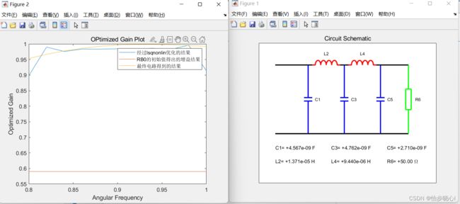
plot(WBR,TPG,WBR,TPG0,WBR,TPG2)
xlabel('Angular Frequency')
ylabel('Optimized Gain')
title('OPtimized Gain Plot')
legend('经过lsqnonlin优化的结果','RB0的初始值得出的增益结果','最终电路得到的结果')
disp(['电路拟合误差为',num2str(resnorm)])

运行结果：

2、验证

电路构建：

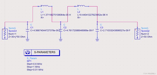
匹配良好：