第2章 Python 数字图像处理(DIP) --数字图像基础5 -- 算术运算、集合、几何变换、傅里叶变换等

数字图像处理所有的基本数字工具介绍

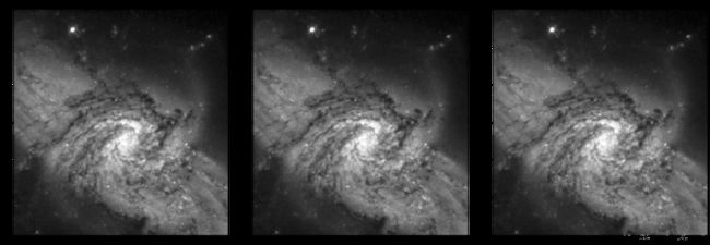
算术运算

# 相加
img_ori = cv2.imread("DIP_Figures/DIP3E_Original_Images_CH02/Fig0226(galaxy_pair_original).tif", 0)

dst = np.zeros_like(img_ori, dtype=float)

for i in range(100):
    dst += img_ori

dst_1000 = np.zeros_like(img_ori, dtype=float)
for i in range(1000):
    dst_1000 += img_ori

plt.figure(figsize=(24, 8))
plt.subplot(1,3,1), plt.imshow(img_ori, 'gray'), plt.title("Original"),# plt.xticks([]), plt.yticks([])
plt.subplot(1,3,2), plt.imshow(dst, 'gray'), plt.title("100"),# plt.xticks([]), plt.yticks([])
plt.subplot(1,3,3), plt.imshow(dst_1000, 'gray'), plt.title("1000"),# plt.xticks([]), plt.yticks([])
plt.tight_layout()
plt.show()

def set_bin_last_0(x):
    """
    这是把最低位为1的有效位置为0， 如：[1, 0, 0, 1, 0, 0] -> [1, 0, 0, 0, 0, 0]
    """
    bin_list = list(bin(x)[2:])
    for i in range(len(bin_list)-1, -1, -1):
        if int(bin_list[i]) == 1:
            bin_list[i] = '0'
            break
    b = "".join(bin_list)
    return int(b, 2)

def set_bin_last_0(x):
    """
    这是把最后一位是1的置为0
    """
    bin_tmp = bin(x)[2:]
    if int(bin_tmp[-1]) == 1:
        string = str(int(bin_tmp) - 1)
        return int(string, 2)
    else:
        return x

# 使用图像想减比较图像
img_ori = cv2.imread("DIP_Figures/DIP3E_Original_Images_CH02/Fig0227(a)(washington_infrared).tif", 0)
img_ori = np.uint8(normalize(img_ori) * 255)

height, width = img_ori.shape[:2]
dst = np.zeros([height, width], dtype=np.uint8)
for h in range(height):
    for w in range(width):
        dst[h, w] = set_bin_last_0(img_ori[h, w])

dst = np.uint8(normalize(dst) * 255)
        
img_diff = img_ori - dst
img_diff = np.uint8(normalize(img_diff) * 255)

plt.figure(figsize=(24, 8))
plt.subplot(1,3,1), plt.imshow(img_ori, 'gray'), plt.title("Original"),# plt.xticks([]), plt.yticks([])
plt.subplot(1,3,2), plt.imshow(dst, 'gray'), plt.title("Set bin last 0"),# plt.xticks([]), plt.yticks([])
plt.subplot(1,3,3), plt.imshow(img_diff, 'gray'), plt.title("Difference"),# plt.xticks([]), plt.yticks([])
plt.tight_layout()
plt.show()

# 使用图像相减比较图像，得到的结果跟书上相去甚远，还得继续研究
img_a = cv2.imread("DIP_Figures/DIP3E_Original_Images_CH02/Fig0228(a)(angiography_mask_image).tif", 0)
img_b = cv2.imread("DIP_Figures/DIP3E_Original_Images_CH02/Fig0228(b)(angiography_live_ image).tif", 0)

img_a = np.uint8(normalize(img_a) * 255)
img_b = np.uint8(normalize(img_b) * 255)

img_diff = (img_a - img_b)

# 锐化算子，锐化内核强调在相邻的像素值的差异，这使图像看起来更生动
kernel_shapen = np.array((
                    [0,-1,0],
                    [-1,5,-1],
                    [0,-1,0]), np.int8)
imgkernel_shapen = cv2.filter2D(img_b, -1, kernel_shapen)
img_diff_sha = imgkernel_shapen - img_a

plt.figure(figsize=(12, 12))
plt.subplot(2,2,1), plt.imshow(img_a, 'gray'), plt.title("Mask"),# plt.xticks([]), plt.yticks([])
plt.subplot(2,2,2), plt.imshow(img_b, 'gray'), plt.title("Live"),# plt.xticks([]), plt.yticks([])
plt.subplot(2,2,3), plt.imshow(img_diff, 'gray'), plt.title("Difference"),# plt.xticks([]), plt.yticks([])
plt.subplot(2,2,4), plt.imshow(img_diff_sha, 'gray'), plt.title("Difference"),# plt.xticks([]), plt.yticks([])
plt.tight_layout()
plt.show()

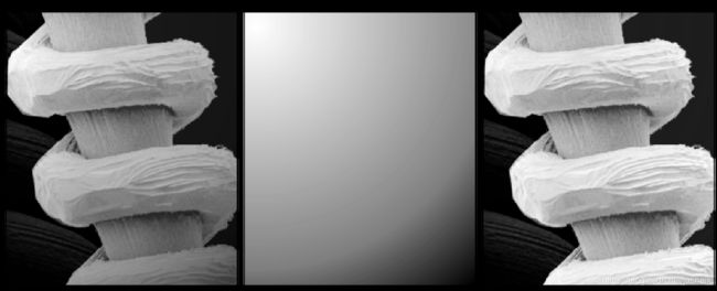
# 使用图像相乘/相除校正阴影和模板
img_a = cv2.imread("DIP_Figures/DIP3E_Original_Images_CH02/Fig0229(a)(tungsten_filament_shaded).tif", 0)
img_b = cv2.imread("DIP_Figures/DIP3E_Original_Images_CH02/Fig0229(b)(tungsten_sensor_shading).tif", 0)
img_dst = img_a / img_b
plt.figure(figsize=(18, 8))
plt.subplot(1,3,1), plt.imshow(img_a, 'gray'), plt.title("Image A"), plt.xticks([]), plt.yticks([])
plt.subplot(1,3,2), plt.imshow(img_b, 'gray'), plt.title("Image B"), plt.xticks([]), plt.yticks([])
plt.subplot(1,3,3), plt.imshow(img_dst, 'gray'), plt.title("Calibration"), plt.xticks([]), plt.yticks([])
plt.tight_layout()
plt.show()

def generatePattern(CheckerboardSize, Nx_cor, Ny_cor):
    '''
    自定义生成棋盘
    :param CheckerboardSize: 棋盘格大小,此处100即可
    :param Nx_cor: 棋盘格横向内角数
    :param Ny_cor: 棋盘格纵向内角数
    :return:
    '''
    black = np.zeros((CheckerboardSize, CheckerboardSize, 3), np.uint8)
    white = np.zeros((CheckerboardSize, CheckerboardSize, 3), np.uint8)
    black[:] = [0, 0, 0]  # 纯黑色
    white[:] = [255, 255, 255]  # 纯白色
 
    black_white = np.concatenate([black, white], axis=1)
    black_white2 = black_white
    white_black = np.concatenate([white, black], axis=1)
    white_black2 = white_black
 
    # 横向连接
    if Nx_cor % 2 == 1:
        for i in range(1, (Nx_cor+1) // 2):
            black_white2 = np.concatenate([black_white2, black_white], axis=1)
            white_black2 = np.concatenate([white_black2, white_black], axis=1)
    else:
        for i in range(1, Nx_cor // 2):
            black_white2 = np.concatenate([black_white2, black_white], axis=1)
            white_black2 = np.concatenate([white_black2, white_black], axis=1)
        black_white2 = np.concatenate([black_white2, black], axis=1)
        white_black2 = np.concatenate([white_black2, white], axis=1)
 
    jj = 0
    black_white3 = black_white2
    for i in range(0, Ny_cor):
        jj += 1
        # 纵向连接
        if jj % 2 == 1:
            black_white3 = np.concatenate((black_white3, white_black2))  # =np.vstack((img1, img2))
        else:
            black_white3 = np.concatenate((black_white3, black_white2))  # =np.vstack((img1, img2))
 
    return black_white3

# 使用图像相乘/相除校正阴影和模板
img_b = cv2.imread("DIP_Figures/DIP3E_Original_Images_CH02/Fig0229(b)(tungsten_sensor_shading).tif", 0)

check = generatePattern(150, 6, 10)
img_temp = check[..., 0][:img_b.shape[0], :img_b.shape[1]].astype(float)
img_temp = img_temp * img_b

img_dst = img_temp / img_b

plt.figure(figsize=(20, 8))
plt.subplot(1,3,1), plt.imshow(img_temp, 'gray'), plt.title("Image A"), plt.xticks([]), plt.yticks([])
plt.subplot(1,3,2), plt.imshow(img_b, 'gray'), plt.title("Image B"), plt.xticks([]), plt.yticks([])
plt.subplot(1,3,3), plt.imshow(img_dst, 'gray'), plt.title("Calibration"), plt.xticks([]), plt.yticks([])
plt.tight_layout()
plt.show()

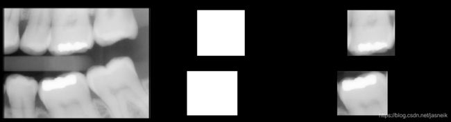
# 使用图像相乘/相除校正阴影和模板
img_a = cv2.imread("DIP_Figures/DIP3E_Original_Images_CH02/Fig0230(a)(dental_xray).tif", 0)
img_b = cv2.imread("DIP_Figures/DIP3E_Original_Images_CH02/Fig0230(b)(dental_xray_mask).tif", 0)
img_temp = normalize(img_b)
img_dst = img_a * img_temp
plt.figure(figsize=(18, 8))
plt.subplot(1,3,1), plt.imshow(img_a, 'gray'), plt.title("Image A"), plt.xticks([]), plt.yticks([])
plt.subplot(1,3,2), plt.imshow(img_b, 'gray'), plt.title("Image B"), plt.xticks([]), plt.yticks([])
plt.subplot(1,3,3), plt.imshow(img_dst, 'gray'), plt.title("Calibration"), plt.xticks([]), plt.yticks([])
plt.tight_layout()
plt.show()

注意

大多数图像是使用不比特显示的（24比特彩色图像由三个不同的8比特通道组成）。因此，我们期望图像的灰度值范围为0 ~ 255。当图像心师傅晚上他啊如TIFF或JPEG存储时，图像的灰度值会自动转换到这一范围。当图像的灰度超过这一允许范围时就会进行剪切或缩放。许多软件 包在把图像转换为8比特时，只是简单地把所有负值转换为0，而把超过这一限值的值转换为255。已知一个或多个算术（或其他）运算产生的数字图像$g$时，保证将一个值的全部范围“捕获”到某个固定比特的方法如下。
$$g_m=g-g_{min}\text{\hspace{1em}(2.31)}$$
然后执行
$$g_s=K[g_m/g_{max}]\text{\hspace{1em}(2.32)}$$
它生成一幅缩放的图像$g_s$，该图像的值域为[0, K]。处理8比特图像时令K=255。执行除法运算时，需要在加上一个较小的数，以免费出现 除以0的现象。

集合运算和逻辑运算

• 补集
  令灰度图像的元素由集合$A$表示，集合$A$的元素形式是三元组$(x,y,z)$，其中$x和y$是空间坐标，$z$是灰度值。我们将集合$A$的补集定义为
  $$A^c=\{(x,y,K-z)|(x,y,z)\in A\}$$
  它是集合$A$中灰度已送去常数K的像素集合。这个常数等于图像中的最大灰度值$2^k -1 $，其中$k$是用于表示$z$的比特数。

• 并集
  元素数量是每个人两个灰度集合A和B的并集定义为：
  $$A\bigcup B=\{\text{max}(a,b)|a\in A,b\in B\}$$

# 补集，并集
img_a = cv2.imread("DIP_Figures/DIP3E_Original_Images_CH02/Fig0232(a)(partial_body_scan).tif", 0)
img_b = 255 - img_a

img_dst = np.zeros(img_a.shape[:2], dtype=np.float)
height, width = img_a.shape[:2]
z = 3 * np.sum(img_a) / (img_a.size)
for i in range(height):
    for j in range(width):
        img_dst[i, j] = max(img_a[i, j], z)

plt.figure(figsize=(15, 10))
plt.subplot(1,3,1), plt.imshow(img_a, 'gray'), plt.title("Image A"), plt.xticks([]), plt.yticks([])
plt.subplot(1,3,2), plt.imshow(img_b, 'gray'), plt.title("Image B"), plt.xticks([]), plt.yticks([])
plt.subplot(1,3,3), plt.imshow(img_dst, 'gray'), plt.title("Calibration"), plt.xticks([]), plt.yticks([])
plt.tight_layout()
plt.show()

逻辑运算

AND、OR、NOT、XOR

def b1_and_b2(img_b1, img_b2):
    """
    input two [0, 1] images, return a [0, 1] image of both images AND operation
    """
    height, width = img_b1.shape[:2]
    img_dst = np.zeros([height, width], np.uint)
    for h in range(height):
        for w in range(width):
            img_dst[h, w] = img_b1[h, w] and img_b2[h, w]
    return img_dst

def b1_or_b2(img_b1, img_b2):
    """
    input two [0, 1] images, return a [0, 1] image of both images OR operation
    """
    height, width = img_b1.shape[:2]
    img_dst = np.zeros([height, width], np.uint)
    for h in range(height):
        for w in range(width):
            img_dst[h, w] = img_b1[h, w] or img_b2[h, w]
    return img_dst

def b1_xor_b2(img_b1, img_b2):
    """
    input two [0, 1] images, return a [0, 1] image of both images XOR operation
    """
    height, width = img_b1.shape[:2]
    img_dst = np.zeros([height, width], np.uint)
    for h in range(height):
        for w in range(width):
            img_dst[h, w] = img_b1[h, w] ^ img_b2[h, w]
    return img_dst

# 逻辑运行
height, width = 300, 400
mid_h, mid_w = height//2 + 1, width//2 + 1

img_b1 = np.zeros([height, width], dtype=np.uint)
img_b1[100:200, 50:250] = 1
img_b2 = np.zeros_like(img_b1, dtype=np.uint)
img_b2[50:150, 150:300] = 1

img_notb1 = normalize(~(img_b1))                  # np.invert  
img_b1_and_b2 = b1_and_b2(img_b1, img_b2)         # b1 AND b2
img_b1_or_b2 = b1_or_b2(img_b1, img_b2)           # b1 OR b2
img_not_b2 = np.uint(normalize(~(img_b2)) + 0.1)  # First NOT img_b2, but return[-2, 0], normalize to [0. 0.9999], +0.1 then conver to [0, 1]
img_b1_and_not_b2 = b1_and_b2(img_b1, img_not_b2) # img_b1 AND NOT(img_b2)
img_b1_xor_b2 = b1_xor_b2(img_b1, img_b2)         # b2 XOR b2


plt.figure(figsize=(7.2, 10))
plt.subplot(5, 3, 2), plt.imshow(img_b1, 'gray'), plt.title('B1'), plt.xticks([]), plt.yticks([])
plt.subplot(5, 3, 3), plt.imshow(img_notb1, 'gray'), plt.title('NOT(B1)'), plt.xticks([]), plt.yticks([])
plt.subplot(5, 3, 4), plt.imshow(img_b1, 'gray'), plt.title('B1'), plt.xticks([]), plt.yticks([])
plt.subplot(5, 3, 5), plt.imshow(img_b2, 'gray'), plt.title('B2'), plt.xticks([]), plt.yticks([])
plt.subplot(5, 3, 6), plt.imshow(img_b1_and_b2, 'gray'), plt.title('B1 AND B2'), plt.xticks([]), plt.yticks([])
plt.subplot(5, 3, 7), plt.imshow(img_b1, 'gray'), plt.title('B1'), plt.xticks([]), plt.yticks([])
plt.subplot(5, 3, 8), plt.imshow(img_b2, 'gray'), plt.title('B2'), plt.xticks([]), plt.yticks([])
plt.subplot(5, 3, 9), plt.imshow(img_b1_or_b2, 'gray'), plt.title('B1 OR B2'), plt.xticks([]), plt.yticks([])
plt.subplot(5, 3, 10), plt.imshow(img_b1, 'gray'), plt.title('B1'), plt.xticks([]), plt.yticks([])
plt.subplot(5, 3, 11), plt.imshow(img_not_b2, 'gray'), plt.title('NOT(B2)'), plt.xticks([]), plt.yticks([])
plt.subplot(5, 3, 12), plt.imshow(img_b1_and_not_b2, 'gray'), plt.title('B1 AND [NOT B2]'), plt.xticks([]), plt.yticks([])
plt.subplot(5, 3, 13), plt.imshow(img_b1, 'gray'), plt.title('B1'), plt.xticks([]), plt.yticks([])
plt.subplot(5, 3, 14), plt.imshow(img_b2, 'gray'), plt.title('B2'), plt.xticks([]), plt.yticks([])
plt.subplot(5, 3, 15), plt.imshow(img_b1_xor_b2, 'gray'), plt.title('B1 XOR B2'), plt.xticks([]), plt.yticks([])
plt.tight_layout()
plt.show()

空间运算

空间运算直接对图像的像素执行，分三类

• （1）单像素运算；

• （2）邻域运算；

• （3）几何空间变换。

• 单像素运算

• 用一个变换同函数$T$改变图像各个像素的灰度，z是原图像中的像素的灰度，s是处理后图像中对应像素（映射）灰度：
  $$s=T(z)\text{\hspace{1em}(2.42)}$$

• 邻域运算

• 邻域处理在输出图像$g$中相同坐标处生成一个对应的像素，这个像素的值由输入图像中邻域尚未确认规定运算和集合$S_{xy}$中的坐标确。如算术平均等。
  $$g(x,y)=\frac{1}{mn}\sum _{(r,c)\in S_{xy}}f(r,c)\text{\hspace{1em}(2.43)}$$

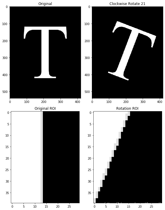
• 几何变换

• 几何变换改变图像中像素的空间排列。这些变换通常称为橡皮膜变换。数字图像的几何变换由两种基本运算组成：

  • （1）坐标的空间变换；
  • （2）灰度内插，即为空间变换后的像素赋灰度值。

• 仿射变换，包括绽放变换、平移变换、旋转变换和剪切变换。
  $$\left[\begin{array}{c}{x}^{\prime }\\ y^{\prime }\end{array}\right]=T\left[\begin{array}{c}x\\ y\end{array}\right]=\left[\begin{array}{cc}{t}_{11}& t_{12}\\ t_{21}& t_{22}\end{array}\right]\left[\begin{array}{c}x\\ y\end{array}\right]\text{\hspace{1em}(2.44)}$$

• 采用如下$3 \times 3 $矩阵，用齐次坐标来表示所有4个仿射变换是可能的
  $$\left[\begin{array}{c}{x}^{\prime }\\ y^{\prime }\\ 1\end{array}\right]=A\left[\begin{array}{c}x\\ y\\ 1\end{array}\right]=\left[\begin{array}{ccc}{a}_{11}& a_{12}& a_{13}\\ a_{21}& a_{22}& a_{23}\\ 0& 0& 1\end{array}\right]\left[\begin{array}{c}x\\ y\\ 1\end{array}\right]\text{\hspace{1em}(2.45)}$$

仿射变换矩阵A

• 恒等 $x^{\prime }=x,y^{\prime }=y$
  $$\left[\begin{array}{ccc}1& 0& 0\\ 0& 1& 0\\ 0& 0& 1\end{array}\right]$$

• 缩入/反射（对于反射，将一个比例因子设为-1，而将另一个比例因子设为0） $x^{\prime }=c_{x}x,y^{\prime }=c_{x}y$
  $$\left[\begin{array}{ccc}{c}_x& 0& 0\\ 0& c_y& 0\\ 0& 0& 1\end{array}\right]$$

• 关于原点旋转$x^{\prime }=xcos\theta -ysin\theta ,y^{\prime }=xsin\theta +ycos\theta$
  $$\left[\begin{array}{ccc}cos\theta & -sin\theta & 0\\ sin\theta & cos\theta & 0\\ 0& 0& 1\end{array}\right]$$

• 平移 $x^{\prime }=x+t_x,y^{\prime }=y+t_y$
  $$\left[\begin{array}{ccc}1& 0& t_x\\ 0& 1& t_y\\ 0& 0& 1\end{array}\right]$$

• 垂直剪切 $x^{\prime }=x+s_{v}y,y^{\prime }=y$
  $$\left[\begin{array}{ccc}1& s_v& 0\\ 0& 1& 0\\ 0& 0& 1\end{array}\right]$$

• 水平剪切 $x^{\prime }=xy,y^{\prime }=y+s_h$
  $$\left[\begin{array}{ccc}1& 0& 0\\ s_h& 1& 0\\ 0& 0& 1\end{array}\right]$$

• 正向映射

• 它包括扫描输入图像的像素，并在每个位置$(x,y)$用式(2.45)直接计算输出图像中相应像素的空间位置$(x^{\prime },y^{\prime })$

• 正向映射的问题是，输入图像中的两个或多个像素可变换到输出图像中的同一位置，这就产生了如何把多个输出值合并为单个输出像素值的问题。

• 另外，某些输出位置可能根本没有要赋值的像素。

• 反射映射

• 它扫描输出像素的位置，并在每个位置$(x^{\prime },y^{\prime })$使用$(x,y)=A^{-1}(x^{\prime },y^{\prime })$计算输入图像中的相应位置，然后在最近的输入像素之间进行内插，求出输出像素的灰度

• 反向映射要比正向映射更有效

# 单像素运算 --> 负图像 : 255 - img
img = cv2.imread('DIP_Figures/DIP3E_Original_Images_CH02/Fig0220(a)(chronometer 3692x2812  2pt25 inch 1250 dpi).tif', 0)
img = img[1100:3500, 200:2600]

x = np.arange(255)
y = 255 - x

img_inv = 255 - img

plt.figure(figsize=(18, 6))
plt.subplot(131), plt.imshow(img, 'gray'), plt.title('Original'), #plt.xticks([]), plt.yticks([])
plt.subplot(132), plt.plot(x, y), plt.title('s = T(z)'), plt.xticks([0, 255]), plt.yticks([0, 255])
plt.subplot(133), plt.imshow(img_inv, 'gray'), plt.title('255 - Image'), #plt.xticks([]), plt.yticks([])
plt.tight_layout()
plt.show()

import numpy as np

def arithmentic_mean(image, kernel):
    """
    caculate image arithmetic mean 
    :param image: input image
    :param kernel: input kernel
    :return: image after convolution
    """
    
    img_h = image.shape[0]
    img_w = image.shape[1]

    m = kernel.shape[0]
    n = kernel.shape[1]

    # padding
    padding_h = int((m -1)/2)
    padding_w = int((n -1)/2)

    image_pad = np.pad(image.copy(), (padding_h, padding_w), mode="constant", constant_values=0)

    image_convol = image.copy().astype(np.float)
    for i in range(padding_h, img_h + padding_h):
        for j in range(padding_w, img_w + padding_w):
            temp = np.sum(image_pad[i-padding_h:i+padding_h+1, j-padding_w:j+padding_w+1] * kernel)
            image_convol[i - padding_h][j - padding_w] = 1/(m * n) * temp

    return image_convol

# 算术平均，m = n = 41
img_ori = cv2.imread('DIP_Figures/DIP3E_Original_Images_CH02/Fig0235(c)(kidney_original).tif', 0) #直接读为灰度图像

m, n = 41, 41
mean_kernal = np.ones([m, n])
mean_kernal = mean_kernal / mean_kernal.size

img_dst = arithmentic_mean(img_ori, kernel=mean_kernal)
img_dst = np.uint8(normalize(img_dst) * 255)
img_cv2_mean = cv2.filter2D(img_ori, ddepth= -1, kernel=mean_kernal)
plt.figure(figsize=(24, 12))

plt.subplot(131), plt.imshow(img_ori, 'gray'), plt.title('Original')
plt.subplot(132), plt.imshow(img_dst, 'gray'), plt.title('Self Mean')
plt.subplot(133), plt.imshow(img_cv2_mean, 'gray'), plt.title('CV2 mean')
plt.tight_layout()
plt.show()

def rotate_image(img, angle=45):
    height, width = img.shape[:2]
    if img.ndim == 3:
        channel = 3
    else:
        channel = None
        
    if int(angle / 90) % 2 == 0:
        reshape_angle = angle % 90
    else:
        reshape_angle = 90 - (angle % 90)
    reshape_radian = np.radians(reshape_angle)  # 角度转弧度
    # 三角函数计算出来的结果会有小数，所以做了向上取整的操作。
    new_height = int(np.ceil(height * np.cos(reshape_radian) + width * np.sin(reshape_radian)))
    new_width = int(np.ceil(width * np.cos(reshape_radian) + height * np.sin(reshape_radian)))
    if channel:
        new_img = np.zeros((new_height, new_width, channel), dtype=np.uint8)
    else:
        new_img = np.zeros((new_height, new_width), dtype=np.uint8)

    radian = np.radians(angle)
    cos_radian = np.cos(radian)
    sin_radian = np.sin(radian)
    # dx = 0.5 * new_width + 0.5 * height * sin_radian - 0.5 * width * cos_radian
    # dy = 0.5 * new_height - 0.5 * width * sin_radian - 0.5 * height * cos_radian
    # ---------------前向映射--------------------
    # for y0 in range(height):
    #     for x0 in range(width):
    #         x = x0 * cos_radian - y0 * sin_radian + dx
    #         y = x0 * sin_radian + y0 * cos_radian + dy
    #         new_img[int(y) - 1, int(x) - 1] = img[int(y0), int(x0)]  # 因为整体映射的结果会比偏移一个单位，所以这里x,y做减一操作。

    # ---------------后向映射--------------------
    dx_back = 0.5 * width - 0.5 * new_width * cos_radian - 0.5 * new_height * sin_radian
    dy_back = 0.5 * height + 0.5 * new_width * sin_radian - 0.5 * new_height * cos_radian
    for y in range(new_height):
        for x in range(new_width):
            x0 = x * cos_radian + y * sin_radian + dx_back
            y0 = y * cos_radian - x * sin_radian + dy_back
            if 0 < int(x0) <= width and 0 < int(y0) <= height:  # 计算结果是这一范围内的x0，y0才是原始图像的坐标。
                new_img[int(y), int(x)] = img[int(y0) - 1, int(x0) - 1]  # 因为计算的结果会有偏移，所以这里做减一操作。


    # # ---------------双线性插值--------------------
    # if channel:
    #     fill_height = np.zeros((height, 2, channel), dtype=np.uint8)
    #     fill_width = np.zeros((2, width + 2, channel), dtype=np.uint8)
    # else:
    #     fill_height = np.zeros((height, 2), dtype=np.uint8)
    #     fill_width = np.zeros((2, width + 2), dtype=np.uint8)
    # img_copy = img.copy()
    # # 因为双线性插值需要得到x+1，y+1位置的像素，映射的结果如果在最边缘的话会发生溢出，所以给图像的右边和下面再填充像素。
    # img_copy = np.concatenate((img_copy, fill_height), axis=1)
    # img_copy = np.concatenate((img_copy, fill_width), axis=0)
    # for y in range(new_height):
    #     for x in range(new_width):
    #         x0 = x * cos_radian + y * sin_radian + dx_back
    #         y0 = y * cos_radian - x * sin_radian + dy_back
    #         x_low, y_low = int(x0), int(y0)
    #         x_up, y_up = x_low + 1, y_low + 1
    #         u, v = np.modf(x0)[0], np.modf(y0)[0]  # 求x0和y0的小数部分
    #         x1, y1 = x_low, y_low
    #         x2, y2 = x_up, y_low
    #         x3, y3 = x_low, y_up
    #         x4, y4 = x_up, y_up
    #         if 0 < int(x0) <= width and 0 < int(y0) <= height:
    #             pixel = (1 - u) * (1 - v) * img_copy[y1, x1] + (1 - u) * v * img_copy[y2, x2] + u * (1 - v) * img_copy[y3, x3] + u * v * img_copy[y4, x4]  # 双线性插值法，求像素值。
    #             new_img[int(y), int(x)] = pixel
    
    return new_img

# 几何空间变换
img_ori = cv2.imread('DIP_Figures/DIP3E_Original_Images_CH02/Fig0236(a)(letter_T).tif', 0) #直接读为灰度图像

height, width = img_ori.shape[:2]

img_21 = np.zeros([height, width], np.uint8)
img_temp = rotate_image(img_ori, 21)
mid_h, mid_w = img_temp.shape[0] // 2 + 1, img_temp.shape[1] // 2 + 1
img_21 = img_temp[mid_h-height//2:mid_h+height//2, mid_w-width//2:mid_w+width//2]

img_roi    = img_ori[210:250, 217:247]
img_21_roi = img_21[210:250, 240:270]

plt.figure(figsize=(8, 10))
plt.subplot(221), plt.imshow(img_ori, 'gray'), plt.title('Original')
plt.subplot(222), plt.imshow(img_21, 'gray'), plt.title('Clockwise Rotate 21')
plt.subplot(223), plt.imshow(img_roi, 'gray'), plt.title('Original ROI')
plt.subplot(224), plt.imshow(img_21_roi, 'gray'), plt.title('Rotation ROI')
plt.tight_layout()
plt.show()

图像配准

图像配准是一种重要的数字图像处理应用，它用于对齐同一场景的两幅或多幅图像。一幅输入图像和一幅参考图像，目的是对输入图像做几何变换，使得输出图像与参考图像对齐（配准）

def sift_kp(img):
    sift = cv2.xfeatures2d.SIFT_create()
    kp, des = sift.detectAndCompute(img, None)
    kp_img = cv2.drawKeypoints(img, kp, None)
    return kp_img, kp, des

def get_good_match(des1, des2):
    bf = cv2.BFMatcher()
    matches = bf.knnMatch(des1, des2, k=2)
    good = []
    for m, n in matches:
        if m.distance < 0.75 * n.distance:
            good.append(m)
    return good

# H, status = cv2.findHomography(ptsA, ptsB, cv2.RANSAC, ransacReprojThreshold)
#其中H为求得的单应性矩阵矩阵
#status则返回一个列表来表征匹配成功的特征点。
#ptsA,ptsB为关键点
#cv2.RANSAC, ransacReprojThreshold这两个参数与RANSAC有关

def sift_image_align(img1, img2):
    """
    图像配准
    """
    _, kp1, des1 = sift_kp(img1)
    _, kp2, des2 = sift_kp(img2)
    good_match = get_good_match(des1, des2)
    if len(good_match) > 4:
        ptsA = np.float32([kp1[m.queryIdx].pt for m in good_match]).reshape(-1, 1, 2)
        ptsB = np.float32([kp2[m.trainIdx].pt for m in good_match]).reshape(-1, 1, 2)
        ransacReprojThreshold = 4
        H, status = cv2.findHomography(ptsA, ptsB, cv2.RANSAC, ransacReprojThreshold)
        img_out = cv2.warpPerspective(img2, H, (img1.shape[1], img1.shape[0]), flags=cv2.INTER_LINEAR + cv2.WARP_INVERSE_MAP)
    return img_out, H, status

# 几何空间变换
img_ori = cv2.imread('DIP_Figures/DIP3E_Original_Images_CH02/Fig0237(a)(characters test pattern)_POST.tif', 0) #直接读为灰度图像
h,w=img_ori.shape[:2]
M = np.array([[1, 0.05, 0], [0.4, 1, 0]], np.float32)
img_dst = cv2.warpAffine(img_ori, M, (w+100, h+350), borderValue=0)

img_out, H, status = sift_image_align(img_ori, np.uint8(img_dst))

img_diff = img_ori - img_out

plt.figure(figsize=(10, 10))
plt.subplot(221), plt.imshow(img_ori, 'gray'), plt.title('Original')
plt.subplot(222), plt.imshow(img_dst, 'gray'), plt.title('Perspective')
plt.subplot(223), plt.imshow(img_out, 'gray'), plt.title('Aligned')
plt.subplot(224), plt.imshow(img_diff, 'gray'), plt.title('Aligned differenc against Original')
plt.tight_layout()
plt.show()

向量与矩阵运算

列向量的$a和b$的内积（也称点积）
$$a\cdot b=a^{T}b=a_1{b}_1+a_2{b}_2+\cdots +a_n{b}_n=\sum _{i=1}^n{a}_i{b}_i\text{\hspace{1em}(2.50)}$$

• 欧几里得向量范数，定义为内积的平方根：
  $$\Vert z\Vert =(z^{T}z{)}^{\frac{1}{2}}\text{\hspace{1em}(2.51)}$$

• 点（向量）$z和a$之间的欧几里得距离$D(z,a)$定义为欧几里得向量范数
  $$D(z,a)=\Vert z-a\Vert =[(z-a{)}^T(z-a){]}^{\frac{1}{2}}\text{\hspace{1em}(2.52)}$$

• 像素向量的另一个优点是在线性变换中，可表示为，$A是大小m\times n的矩阵，z和a是大小为n\times 1的列向量$
  $$w=A(z-a)\text{\hspace{1em}(2.53)}$$

• 图像的更广泛的线性处理，$f$是表示$MN\times 1$向量，$n$是表示$M\times N$噪声模式的$MN\times 1$的向量，$g$是表示 处理后图像的$MN\times 1$向量，$H$是表示用于对输入图像进行线性处理的$MN\times MN$矩阵
  $$g=Hf+n\text{\hspace{1em}(2.54)}$$

图像变换

图像处理任务最好按如下步骤完成：

• 变换输入图像
• 在变换域执行规定的任务，
• 执行反变换，
• 返回空间域。

二维线性变换是一种特别重要的变换，其通式为：
$$T(u,v)=\sum _{x=0}^{M-1}\sum _{y=0}^{N-1}f(x,y)r(x,y,u,v)\text{\hspace{1em}(2.55)}$$
$f(x,y)$是输入图像，$r(x,y,u,v)$称为正变换核，$u和v$称为变换量，$T(u,v)称为f(x,y)$的正变换

反变换
$$f(x,y)=\sum _{u=0}^{M-1}\sum _{v=0}^{N-1}T(u,v)s(x,y,u,v)\text{\hspace{1em}(2.56)}$$
$s(x,y,u,v)$称为反变换核

可分离变换核
$$r(x,y,u,v)=r_1(x,u)r_2(y,v)\text{\hspace{1em}(2.57)}$$
对称变换核
$$r(x,y,u,v)=r_1(x,u)r_1(y,v)\text{\hspace{1em}(2.58)}$$

傅里叶变换的正变换核与反变换核
$$r(x,y,u,v)=e^{-j2\pi (ux/M+vy/N)}\text{\hspace{1em}(2.59)}$$
$$s(x,y,u,v)=\frac{1}{MN}{e}^{j2\pi (ux/M+vy/N)}\text{\hspace{1em}(2.60)}$$
傅里叶变换核是可分离的和对称的

def add_sin_noise(img, scale=1, angle=0):
    """
    add sin noise for image
    param: img: input image, 1 channel, dtype=uint8
    param: scale: sin scaler, smaller than 1, will enlarge, bigger than 1 will shrink
    param: angle: angle of the rotation
    return: output_img: output image is [0, 1] image which you could use as mask or any you want to
    """
    
    height, width = img.shape[:2]  # original image shape
    
    # convert all the angle
    if int(angle / 90) % 2 == 0:
        rotate_angle = angle % 90
    else:
        rotate_angle = 90 - (angle % 90)
    
    rotate_radian = np.radians(rotate_angle)    # convert angle to radian
    
    # get new image height and width
    new_height = int(np.ceil(height * np.cos(rotate_radian) + width * np.sin(rotate_radian)))
    new_width = int(np.ceil(width * np.cos(rotate_radian) + height * np.sin(rotate_radian))) 
    
    # if new height or new width less than orginal height or width, the output image will be not the same shape as input, here set it right
    if new_height < height:
        new_height = height
    if new_width < width:
        new_width = width
    
    # meshgrid
    u = np.arange(new_width)
    v = np.arange(new_height)
    u, v = np.meshgrid(u, v)
    
    # get sin noise image, you could use scale to make some difference, better you could add some shift
    noise = abs(np.sin(u * scale))
    
    # here use opencv to get rotation, better write yourself rotation function
    C1=cv2.getRotationMatrix2D((new_width/2.0, new_height/2.0), angle, 1)
    new_img=cv2.warpAffine(noise, C1, (int(new_width), int(new_height)), borderValue=0)
    
    offset_height = abs(new_height - height) // 2
    offset_width = abs(new_width - width) // 2
    img_dst = new_img[offset_height:offset_height + height, offset_width:offset_width+width]
    output_img = (img_dst - img_dst.min()) / (img_dst.max() - img_dst.min())
    
    return output_img 

def butterworth_notch_filter(img, D0, uk, vk, order=1):
    M, N = img.shape[1], img.shape[0]
    
    u = np.arange(M)
    v = np.arange(N)
    
    u, v = np.meshgrid(u, v)
    
    DK = np.sqrt((u - M//2 - uk)**2 + (v - N//2 - vk)**2)
    D_K = np.sqrt((u - M//2 + uk)**2 + (v - N//2 + vk)**2)
    
    kernel = (1 / (1 + (D0 / (DK+1e-5))**order)) * (1 / (1 + (D0 / (D_K+1e-5))**order))
    
    kernel_normal = (kernel - kernel.min()) / (kernel.max() - kernel.min())

    return kernel_normal

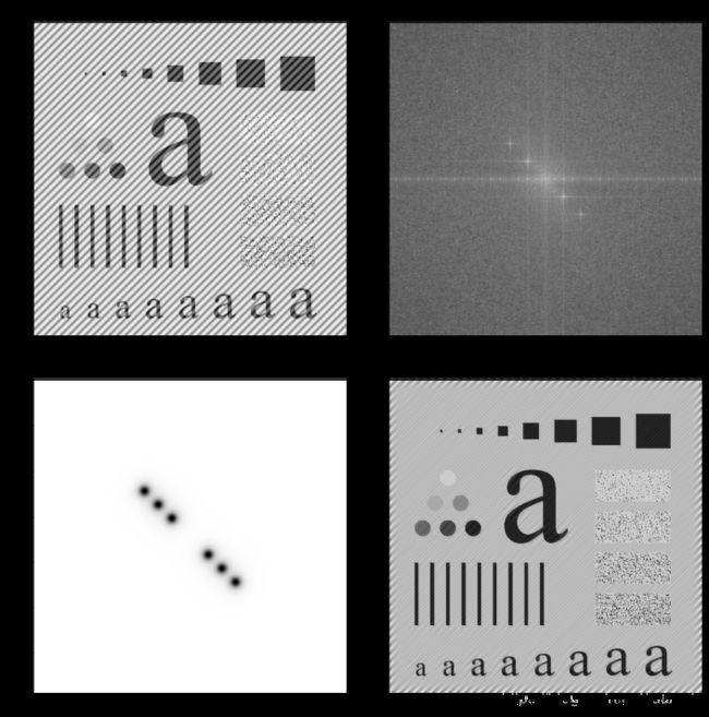
# Sine noise -> denoise
import cv2
import matplotlib.pyplot as plt

# input image without noise
img_ori = cv2.imread('DIP_Figures/DIP3E_Original_Images_CH02/Fig0237(a)(characters test pattern)_POST.tif', 0) #直接读为灰度图像

# sine noise
noise = add_sin_noise(img_ori, scale=0.25, angle=-45)

# image with sine noise
img = np.array(img_ori / 255, np.float32)
img = img + noise

# clip & normalize and set image to 8 bits [0, 255]
img = normalize(img)
img = np.clip(img, low_clip, 1.0)
img = np.uint8(img * 255)

# Denoise with Butterworth notch filter
plt.figure(figsize=(10, 10))
plt.subplot(221),plt.imshow(img,'gray'),plt.title('Image with sin noise')

#--------------------------------
fft = np.fft.fft2(img)
fft_shift = np.fft.fftshift(fft)
amp_img = np.abs(np.log(1 + np.abs(fft_shift)))
plt.subplot(222),plt.imshow(amp_img,'gray'),plt.title('FFT')

#--------------------------------
order = 3
start = 40
step = 30
BNF_dst = 1.0
for i in range(order):
    BNF = butterworth_notch_filter(img, D0=10, uk=start + i * step, vk=start + i * step, order=3)
    BNF_dst *= BNF
plt.subplot(223),plt.imshow((BNF_dst),'gray'),plt.title('mask')

#--------------------------------
# 对新的图像进行逆变换
f1shift = fft_shift * (BNF_dst)
f2shift = np.fft.ifftshift(f1shift) 
img_new = np.fft.ifft2(f2shift)

#出来的是复数，无法显示
img_new = np.abs(img_new)

#调整大小范围便于显示
img_new = np.uint8(normalize(img_new) * 255)
plt.subplot(224),plt.imshow(img_new,'gray'),plt.title('Denoised')

# fft_mask = amp_img * BNF_dst
# plt.subplot(224),plt.imshow(fft_mask,'gray'),plt.title('FFT with mask')

plt.tight_layout()
plt.show()

当正、反变换核可分、对称，且$f(x,y)$是大小为$M\times M$的方形图像时，式（2.55）和式（2.56）可表示为矩阵形式：
$$T=AFA\text{\hspace{1em}(2.63)}$$
反变换：
$$BTB=BAFAB\text{\hspace{1em}(2.64)}$$
若$B=A^{-1}$，则$F=BTB$，完全恢复；若$B\ne A^{-1}$，则$\hat{F}=BAFAB$，近似恢复。

图像和随机变量

灰度级$z_k$在这幅图像中出现的概率
$$p(z_k)=\frac{n_k}{MN}\text{\hspace{1em}(2.67)}$$
$n_k$是灰度级$z_k$在图像中出现的次数
$$\sum _{k=0}^{L-1}p(z_k)=1\text{\hspace{1em}(2.68)}$$

均值（平均）灰度为：
$$m=\sum _{k=0}^{L-1}{z}_{k}p(z_k)\text{\hspace{1em}(2.69)}$$
灰度的方差为：
$${\sigma }^2=\sum _{k=0}^{L-1}(z_k-m{)}^{2}p(z_k)\text{\hspace{1em}(2.70)}$$
第$n$阶中心矩：
灰度的方差为
$${\mu }_n(z)=\sum _{k=0}^{L-1}(z_k-m{)}^{n}p(z_k)\text{\hspace{1em}(2.71)}$$