Python 傅里叶变换 Fourier Transform

Python 傅里叶变换 Fourier Transform

flyfish

0 解释什么是Period 和 Amplitude

import matplotlib.pyplot as plt
import numpy as np

plt.style.use('seaborn-poster')
%matplotlib inline
x = np.linspace(0, 20, 201)
y = np.sin(x)

plt.figure(figsize = (8, 6))
plt.plot(x, y, 'b')
plt.ylabel('Amplitude')
plt.xlabel('Location (x)')
plt.show()

一图胜千言

Fast Fourier Transform (FFT) 快速傅里叶变换
快速傅里叶逆变换

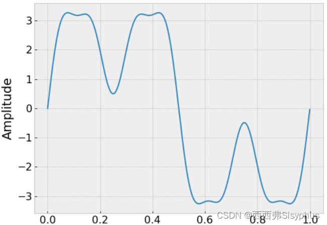
1 在时域中绘制信号

import matplotlib.pyplot as plt
import numpy as np
from scipy.fftpack import fft, ifft
# sampling rate 也叫 Sampling frequency 
sr = 2000
# sampling interval 也叫 Sampling period  
ts = 1.0/sr
t = np.arange(0,1,ts)#start, stop, step #[0.000e+00 5.000e-04 1.000e-03 ... 9.985e-01 9.990e-01 9.995e-01]
#(len(t))==2000

freq_feature = 1
x = 3*np.sin(2*np.pi*freq_feature*t)

freq_feature =3
x += 2*np.sin(2*np.pi*freq_feature*t)

freq_feature = 7
x += 0.5* np.sin(2*np.pi*freq_feature*t)

plt.figure(figsize = (8, 6))
print(len(x))#Length of signal
plt.plot(t, x)
plt.ylabel('Amplitude')

plt.show()

$$period=\frac{1}{frequency}$$

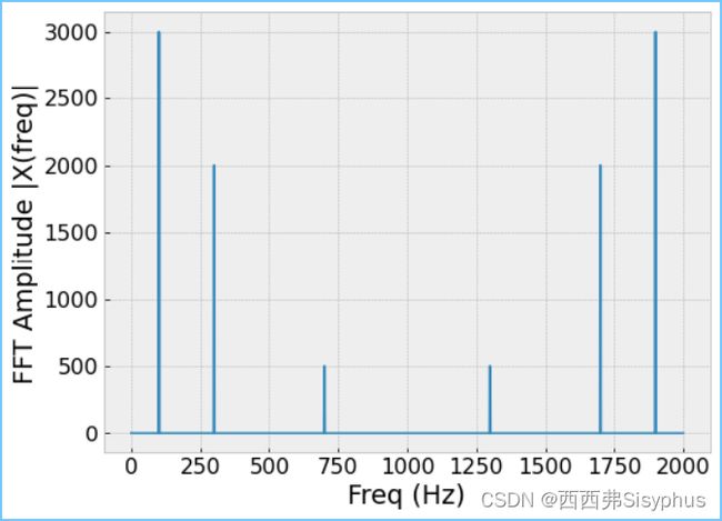
2 绘制快速傅里叶变换图

X = fft(x)
N = len(X)
n = np.arange(N)#[   0    1    2 ... 1997 1998 1999]
T = N/sr
freq = n/T 
X = fft(x)

plt.figure(figsize = (8, 6))

plt.plot(freq, np.abs(X))

plt.xlabel('Freq (Hz)')
plt.ylabel('FFT Amplitude |X(freq)|')

因为1、3、7相对2000，在坐标轴上太小把上述代码freq_feature 改成100,300,700更容易看出特点

freq_feature = 100
x = 3*np.sin(2*np.pi*freq_feature*t)

freq_feature =300
x += 2*np.sin(2*np.pi*freq_feature*t)

freq_feature = 700
x += 0.5* np.sin(2*np.pi*freq_feature*t)

继续绘制freq_feature =1、3、7的傅里叶变换图

plt.figure(figsize = (8, 6))

plt.stem(freq, np.abs(X))
plt.xlim(0, 10)
plt.xlabel('Freq (Hz)')
plt.ylabel('FFT Amplitude |X(freq)|')
plt.show()

这样就看的更清楚了

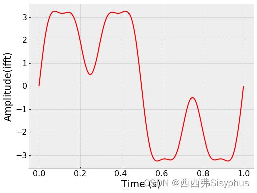
3 通过ifft快速傅里叶逆变换还原数据

plt.figure(figsize = (8, 6))
plt.plot(t, ifft(X), 'r')
plt.xlabel('Time (s)')
plt.ylabel('Amplitude(ifft)')

因为fft之后的结果是对称的所以可以只绘制one-sided

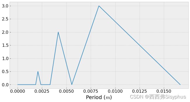
4 可以转换成分钟显示

t_h = 1/f_oneside / (60)
plt.figure(figsize=(8,6))
plt.plot(t_h, np.abs(X[:n_oneside])/n_oneside)
plt.xlabel('Period ($m$)')
plt.show()

5 完整代码

# -*- coding: utf-8 -*-

import matplotlib.pyplot as plt
import numpy as np
from scipy.fftpack import fft, ifft
# sampling rate 也叫 Sampling frequency 
sr = 2000
# sampling interval 也叫 Sampling period  
ts = 1.0/sr
t = np.arange(0,1,ts)#start, stop, step #[0.000e+00 5.000e-04 1.000e-03 ... 9.985e-01 9.990e-01 9.995e-01]
#(len(t))==2000

freq_feature = 1
x = 3*np.sin(2*np.pi*freq_feature*t)

freq_feature =3
x += 2*np.sin(2*np.pi*freq_feature*t)

freq_feature = 7
x += 0.5* np.sin(2*np.pi*freq_feature*t)

plt.figure(figsize = (8, 6))
print(len(x))#Length of signal
plt.plot(t, x)
plt.ylabel('Amplitude')

plt.show()



X = fft(x)
N = len(X)
n = np.arange(N)#[   0    1    2 ... 1997 1998 1999]
T = N/sr
freq = n/T 
X = fft(x)

plt.figure(figsize = (8, 6))

plt.stem(freq, np.abs(X))
plt.xlim(0, 10)
plt.xlabel('Freq (Hz)')
plt.ylabel('FFT Amplitude |X(freq)|')
plt.show()


plt.figure(figsize = (8, 6))
plt.plot(t, ifft(X), 'r')
plt.xlabel('Time (s)')
plt.ylabel('Amplitude(ifft)')



# Get the one-sided specturm
n_oneside = N//2
# get the one side frequency
f_oneside = freq[:n_oneside]+1
print("f_oneside:",f_oneside)

plt.figure(figsize = (12, 6))
plt.plot(f_oneside, np.abs(X[:n_oneside]))
plt.xlabel('Freq (Hz)')
plt.ylabel('FFT Amplitude one-sided')
plt.show()



t_h = 1/f_oneside / (60)
plt.figure(figsize=(8,6))
plt.plot(t_h, np.abs(X[:n_oneside])/n_oneside)
plt.xlabel('Period ($m$)')
plt.show()