LeNet对MNIST 数据集中的图像进行分类--keras实现

我们将训练一个卷积神经网络来对 MNIST 数据库中的图像进行分类，可以与前面所提到的CNN实现对比CNN对 MNIST 数据库中的图像进行分类-CSDN博客

加载 MNIST 数据库

MNIST 是机器学习领域最著名的数据集之一。

• 它有 70,000 张手写数字图像 - 下载非常简单 - 图像尺寸为 28x28 - 灰度图像

from keras.datasets import mnist

# 使用 Keras 导入预洗牌 MNIST 数据库
(X_train, y_train), (X_test, y_test) = mnist.load_data()

print("The MNIST database has a training set of %d examples." % len(X_train))
print("The MNIST database has a test set of %d examples." % len(X_test))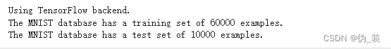

将前六个训练图像可视化 

import matplotlib.pyplot as plt
%matplotlib inline
import matplotlib.cm as cm
import numpy as np

# 绘制前六幅训练图像
fig = plt.figure(figsize=(20,20))
for i in range(6):
    ax = fig.add_subplot(1, 6, i+1, xticks=[], yticks=[])
    ax.imshow(X_train[i], cmap='gray')
    ax.set_title(str(y_train[i]))

 查看图像的更多细节

def visualize_input(img, ax):
    ax.imshow(img, cmap='gray')
    width, height = img.shape
    thresh = img.max()/2.5
    for x in range(width):
        for y in range(height):
            ax.annotate(str(round(img[x][y],2)), xy=(y,x),
                        horizontalalignment='center',
                        verticalalignment='center',
                        color='white' if img[x][y]

预处理输入图像：通过将每幅图像中的每个像素除以 255 来调整图像比例

# normalize the data to accelerate learning
mean = np.mean(X_train)
std = np.std(X_train)
X_train = (X_train-mean)/(std+1e-7)
X_test = (X_test-mean)/(std+1e-7)

print('X_train shape:', X_train.shape)
print(X_train.shape[0], 'train samples')
print(X_test.shape[0], 'test samples')

对标签进行预处理：使用单热方案对分类整数标签进行编码

from keras.utils import np_utils

num_classes = 10 
# print first ten (integer-valued) training labels
print('Integer-valued labels:')
print(y_train[:10])

# one-hot encode the labels
# convert class vectors to binary class matrices
y_train = np_utils.to_categorical(y_train, num_classes)
y_test = np_utils.to_categorical(y_test, num_classes)

# print first ten (one-hot) training labels
print('One-hot labels:')
print(y_train[:10])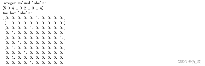

重塑数据以适应我们的 CNN（和 input_shape）

# input image dimensions 28x28 pixel images. 
img_rows, img_cols = 28, 28

X_train = X_train.reshape(X_train.shape[0], img_rows, img_cols, 1)
X_test = X_test.reshape(X_test.shape[0], img_rows, img_cols, 1)
input_shape = (img_rows, img_cols, 1)

print('image input shape: ', input_shape)
print('x_train shape:', X_train.shape)

定义模型架构

论文地址：lecun-01a.pdf

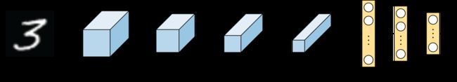
要在 Keras 中实现 LeNet-5，请阅读原始论文并从第 6、7 和 8 页中提取架构信息。以下是构建 LeNet-5 网络的主要启示：

• 每个卷积层的滤波器数量：从图中（以及论文中的定义）可以看出，每个卷积层的深度（滤波器数量）如下：C1 = 6、C3 = 16、C5 = 120 层。
• 每个 CONV 层的内核大小：根据论文，内核大小 = 5 x 5
• 每个卷积层之后都会添加一个子采样层（POOL）。每个单元的感受野是一个 2 x 2 的区域（即 pool_size = 2）。请注意，LeNet-5 创建者使用的是平均池化，它计算的是输入的平均值，而不是我们在早期项目中使用的最大池化层，后者传递的是输入的最大值。如果您有兴趣了解两者的区别，可以同时尝试。在本实验中，我们将采用论文架构。
• 激活函数：LeNet-5 的创建者为隐藏层使用了 tanh 激活函数，因为对称函数被认为比 sigmoid 函数收敛更快。一般来说，我们强烈建议您为网络中的每个卷积层添加 ReLU 激活函数。

需要记住的事项

• 始终为 CNN 中的 Conv2D 层添加 ReLU 激活函数。除了网络中的最后一层，密集层也应具有 ReLU 激活函数。
• 在构建分类网络时，网络的最后一层应该是具有软最大激活函数的密集（FC）层。最终层的节点数应等于数据集中的类别总数。

from keras.models import Sequential
from keras.layers import Conv2D, AveragePooling2D, Flatten, Dense

#Instantiate an empty model
model = Sequential()

# C1 Convolutional Layer
model.add(Conv2D(6, kernel_size=(5, 5), strides=(1, 1), activation='tanh', input_shape=input_shape, padding='same'))

# S2 Pooling Layer
model.add(AveragePooling2D(pool_size=(2, 2), strides=2, padding='valid'))

# C3 Convolutional Layer
model.add(Conv2D(16, kernel_size=(5, 5), strides=(1, 1), activation='tanh', padding='valid'))

# S4 Pooling Layer
model.add(AveragePooling2D(pool_size=(2, 2), strides=2, padding='valid'))

# C5 Fully Connected Convolutional Layer
model.add(Conv2D(120, kernel_size=(5, 5), strides=(1, 1), activation='tanh', padding='valid'))

#Flatten the CNN output so that we can connect it with fully connected layers
model.add(Flatten())

# FC6 Fully Connected Layer
model.add(Dense(84, activation='tanh'))

# Output Layer with softmax activation
model.add(Dense(10, activation='softmax'))

# print the model summary
model.summary()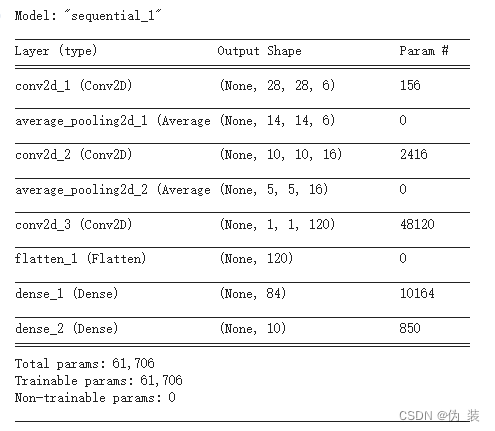

编译模型

我们将使用亚当优化器

# the loss function is categorical cross entropy since we have multiple classes (10) 


# compile the model by defining the loss function, optimizer, and performance metric
model.compile(loss='categorical_crossentropy', optimizer='adam', metrics=['accuracy'])

训练模型

LeCun 和他的团队采用了计划衰减学习法，学习率的值按照以下时间表递减：前两个历元为 0.0005，接下来的三个历元为 0.0002，接下来的四个历元为 0.00005，之后为 0.00001。在论文中，作者对其网络进行了 20 个历元的训练。

from keras.callbacks import ModelCheckpoint, LearningRateScheduler

# set the learning rate schedule as created in the original paper
def lr_schedule(epoch):
    if epoch <= 2:     
        lr = 5e-4
    elif epoch > 2 and epoch <= 5:
        lr = 2e-4
    elif epoch > 5 and epoch <= 9:
        lr = 5e-5
    else: 
        lr = 1e-5
    return lr

lr_scheduler = LearningRateScheduler(lr_schedule)

# set the checkpointer
checkpointer = ModelCheckpoint(filepath='model.weights.best.hdf5', verbose=1, 
                               save_best_only=True)

# train the model
hist = model.fit(X_train, y_train, batch_size=32, epochs=20,
          validation_data=(X_test, y_test), callbacks=[checkpointer, lr_scheduler], 
          verbose=2, shuffle=True)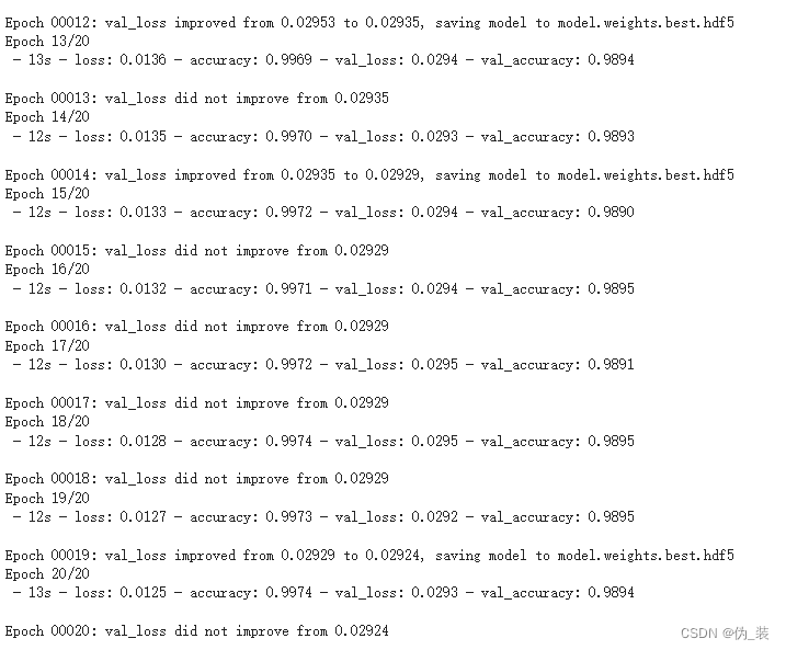

在验证集上加载分类准确率最高的模型

# load the weights that yielded the best validation accuracy
model.load_weights('model.weights.best.hdf5')

计算测试集的分类准确率

# evaluate test accuracy
score = model.evaluate(X_test, y_test, verbose=0)
accuracy = 100*score[1]

# print test accuracy
print('Test accuracy: %.4f%%' % accuracy)

评估模型

import matplotlib.pyplot as plt

f, ax = plt.subplots()
ax.plot([None] + hist.history['accuracy'], 'o-')
ax.plot([None] + hist.history['val_accuracy'], 'x-')
# 绘制图例并自动使用最佳位置： loc = 0。
ax.legend(['Train acc', 'Validation acc'], loc = 0)
ax.set_title('Training/Validation acc per Epoch')
ax.set_xlabel('Epoch')
ax.set_ylabel('acc')
plt.show()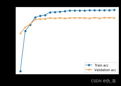

import matplotlib.pyplot as plt

f, ax = plt.subplots()
ax.plot([None] + hist.history['loss'], 'o-')
ax.plot([None] + hist.history['val_loss'], 'x-')

# Plot legend and use the best location automatically: loc = 0.
ax.legend(['Train loss', "Val loss"], loc = 0)
ax.set_title('Training/Validation Loss per Epoch')
ax.set_xlabel('Epoch')
ax.set_ylabel('Loss')
plt.show()