【Keras-MLP-GAN】MNIST

原文

本博客是 One Day One GAN_keras版 [DAY 1] 的 learning notes！把代码梳理了一遍，用自己喜欢的方式呈现出来了！GAN 是用 MLP 搭建的！！！

---

---

1 GAN 的前世今生

生成对抗网络（英语：Generative Adversarial Network，简称GAN）是非监督式学习的一种方法，通过让两个神经网络相互博弈的方式进行学习。该方法由伊恩·古德费洛等人于2014年提出。

生成对抗网络由一个生成网络与一个判别网络组成。生成网络从潜在空间（latent space）中随机采样作为输入，其输出结果需要尽量模仿训练集中的真实样本。判别网络的输入则为真实样本或生成网络的输出，其目的是将生成网络的输出从真实样本中尽可能分辨出来。而生成网络则要尽可能地欺骗判别网络。两个网络相互对抗、不断调整参数，最终目的是使判别网络无法判断生成网络的输出结果是否真实。

GAN就是把一个随机变量的分布映射到我们给定的数据集的分布：

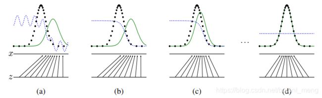
1）基本框架如下：

2）核心公式

• 先看前部分 max D
  
  第一项 D(x) 越大越好，是希望判别器能很好的识别 x 为 true
  第二项 D(G(z)) 越小越好，是希望判别器能很好的识别生成的图片为 false

• 再看后部分 min G
  
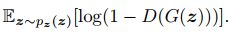
  D(G(z)) 越大越好，希望生成的图片被判别器识别为 true，以假乱真！

3）训练过程

2 GAN 生成 MNIST

代码参考：https://github.com/OUCMachineLearning/OUCML/blob/master/One Day One GAN/day1/gan/gan.py
关于MNIST的介绍和小实验可以参考 【Programming】 的 3.5 或者 3.6 小节！

2.1 导入必要的库

from keras.datasets import mnist
from keras.layers import Input, Dense, Reshape, Flatten, Dropout
from keras.layers import BatchNormalization, Activation, ZeroPadding2D
from keras.layers.advanced_activations import LeakyReLU
from keras.layers.convolutional import UpSampling2D, Conv2D
from keras.models import Sequential, Model
from keras.optimizers import Adam

import matplotlib.pyplot as plt
import matplotlib
matplotlib.use('Agg')
import sys

import numpy as np

2.2 搭建 generator

generator 输入噪声（100），可以产生图片（28，28，1），这里用 MLP 的形式，也即都是 fully connection！

100→256→1024→784→reshape 成 （28,28,1）

# build_generator
model = Sequential()

model.add(Dense(256, input_dim=100))
model.add(LeakyReLU(alpha=0.2))
model.add(BatchNormalization(momentum=0.8))

model.add(Dense(512))
model.add(LeakyReLU(alpha=0.2))
model.add(BatchNormalization(momentum=0.8))
          
model.add(Dense(1024))
model.add(LeakyReLU(alpha=0.2))
model.add(BatchNormalization(momentum=0.8))
          
model.add(Dense(np.prod((28,28,1)), activation='tanh'))
model.add(Reshape((28,28,1)))

model.summary()

noise = Input(shape=(100,)) # input 100,这里写成100不加逗号不行哟
img = model(noise) # output (28,28,1)
        
generator = Model(noise, img)

output

_________________________________________________________________
Layer (type)                 Output Shape              Param #   
=================================================================
dense_1 (Dense)              (None, 256)               25856     
_________________________________________________________________
leaky_re_lu_1 (LeakyReLU)    (None, 256)               0         
_________________________________________________________________
batch_normalization_1 (Batch (None, 256)               1024      
_________________________________________________________________
dense_2 (Dense)              (None, 512)               131584    
_________________________________________________________________
leaky_re_lu_2 (LeakyReLU)    (None, 512)               0         
_________________________________________________________________
batch_normalization_2 (Batch (None, 512)               2048      
_________________________________________________________________
dense_3 (Dense)              (None, 1024)              525312    
_________________________________________________________________
leaky_re_lu_3 (LeakyReLU)    (None, 1024)              0         
_________________________________________________________________
batch_normalization_3 (Batch (None, 1024)              4096      
_________________________________________________________________
dense_4 (Dense)              (None, 784)               803600    
_________________________________________________________________
reshape_1 (Reshape)          (None, 28, 28, 1)         0         
=================================================================
Total params: 1,493,520
Trainable params: 1,489,936
Non-trainable params: 3,584
_________________________________________________________________

参数量的计算这里不在赘述，请参考上面推荐的文章！

2.3 搭建 discriminator

分类网络，输入（28，28，1），输出概率值（sigmoid），也都是用的 MLP

（28，28，1）flatten 为 784→512→256→1

# build_discriminator
model = Sequential()

model.add(Flatten(input_shape=(28,28,1)))

model.add(Dense(512))
model.add(LeakyReLU(alpha=0.2))

model.add(Dense(256))
model.add(LeakyReLU(alpha=0.2))

model.add(Dense(1, activation='sigmoid'))
model.summary()

img = Input(shape=(28,28,1)) # 输入 （28，28，1）
validity = model(img) # 输出二分类结果

discriminator = Model(img, validity)

output

_________________________________________________________________
Layer (type)                 Output Shape              Param #   
=================================================================
flatten_1 (Flatten)          (None, 784)               0         
_________________________________________________________________
dense_5 (Dense)              (None, 512)               401920    
_________________________________________________________________
leaky_re_lu_4 (LeakyReLU)    (None, 512)               0         
_________________________________________________________________
dense_6 (Dense)              (None, 256)               131328    
_________________________________________________________________
leaky_re_lu_5 (LeakyReLU)    (None, 256)               0         
_________________________________________________________________
dense_7 (Dense)              (None, 1)                 257       
=================================================================
Total params: 533,505
Trainable params: 533,505
Non-trainable params: 0
_________________________________________________________________

2.4 compile 模型，对学习过程进行配置

这里训练 GAN 分为两个过程

• 训练 discriminator，图片由固定 generator 产生
• 训练 generator，联合 discriminator 和 generator，但是 discriminator 的梯度不更新，所以 discriminator 固定住了

optimizer = Adam(0.0002, 0.5)

# discriminator
discriminator.compile(loss='binary_crossentropy',
                      optimizer=optimizer,
                      metrics=['accuracy'])


# The combined model  (stacked generator and discriminator)
z = Input(shape=(100,))
img = generator(z)
validity = discriminator(img)
# For the combined model we will only train the generator
discriminator.trainable = False

# Trains the generator to fool the discriminator
combined = Model(z, validity)
combined.summary()
combined.compile(loss='binary_crossentropy', 
                 optimizer=optimizer)

2.5 保存生成的图片

def sample_images(epoch):
    r, c = 5, 5
    noise = np.random.normal(0, 1, (r * c, 100))
    gen_imgs = generator.predict(noise)

    # Rescale images 0 - 1
    gen_imgs = 0.5 * gen_imgs + 0.5

    fig, axs = plt.subplots(r, c)
    cnt = 0
    for i in range(r):
        for j in range(c):
            axs[i,j].imshow(gen_imgs[cnt, :,:,0], cmap='gray')
            axs[i,j].axis('off')
            cnt += 1
    fig.savefig("images/%d.png" % epoch)
    plt.close()

2.6 训练

batch_size 设置为 32，每隔 500 次 iteration（代码中叫 epoch 不太合理），打印一下结果，保存生成的图片！

batch_size = 32
sample_interval = 500

# Load the dataset
(X_train, _), (_, _) = mnist.load_data() # (60000,28,28)
# Rescale -1 to 1
X_train = X_train / 127.5 - 1. # tanh 的结果是 -1~1，所以这里 0-1 归一化后减1
X_train = np.expand_dims(X_train, axis=3)  # (60000,28,28,1)
# Adversarial ground truths
valid = np.ones((batch_size, 1))
fake = np.zeros((batch_size, 1))

for epoch in range(30001):
    # ---------------------
    #  Train Discriminator
    # ---------------------

    # Select a random batch of images
    idx = np.random.randint(0, X_train.shape[0], batch_size) # 0-60000 中随机抽  
    imgs = X_train[idx]
    noise = np.random.normal(0, 1, (batch_size, 100))# 生成标准的高斯分布噪声

    # Generate a batch of new images
    gen_imgs = generator.predict(noise)

    # Train the discriminator
    d_loss_real = discriminator.train_on_batch(imgs, valid) #真实数据对应标签１
    d_loss_fake = discriminator.train_on_batch(gen_imgs, fake) #生成的数据对应标签０
    d_loss = 0.5 * np.add(d_loss_real, d_loss_fake)

    # ---------------------
    #  Train Generator
    # ---------------------
    noise = np.random.normal(0, 1, (batch_size, 100))

    # Train the generator (to have the discriminator label samples as valid)
    g_loss = combined.train_on_batch(noise, valid)

    # Plot the progress
    if epoch % 500==0:
        print ("%d [D loss: %f, acc.: %.2f%%] [G loss: %f]" % (epoch, d_loss[0], 100*d_loss[1], g_loss))

    # If at save interval => save generated image samples
    if epoch % sample_interval == 0:
        sample_images(epoch)

np.random.normal 可以参考博客 python中的np.random.normal

截取了部分 epoch 的结果！

0 [D loss: 0.845254, acc.: 39.06%] [G loss: 0.899815]
500 [D loss: 0.660518, acc.: 68.75%] [G loss: 0.747342]
1000 [D loss: 0.574188, acc.: 71.88%] [G loss: 0.897315]
……

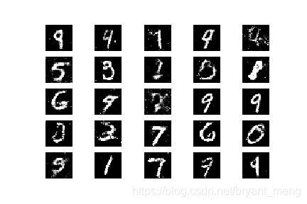
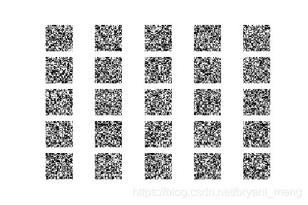
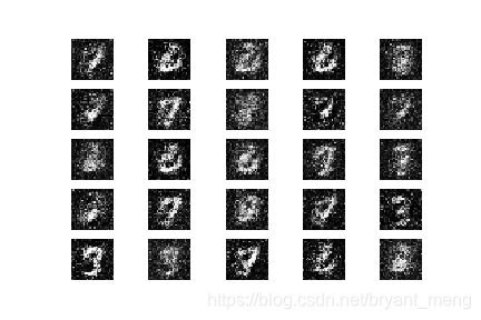
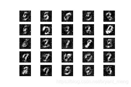
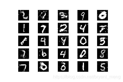
2.7 结果展示

看看生成的图片
0 iteration

500 iteration

1000 iteration

29000 iteration

29500 iteration

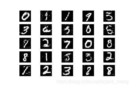
30000 iteration