Manipulating the loss calculation to enhance the training process of physics-informed neural
论文阅读:Manipulating the loss calculation to enhance the training process of physics-informed neural networks to solve the 1D wave equation
- Manipulating the loss calculation to enhance the training process of physics-informed neural networks to solve the 1D wave equation
-
- 定义
-
- PINN定义
- 波动方程
- 失效情况及分析
-
- 驻波
- 具有反射边界和源函数的情况
- 分析
- 解决方法
-
- 对数PDE损失
- S形自适应正则化乘数 λ \lambda λ
- 实验结果
-
- 驻波
- 具有反射边界和源函数的情况
-
- 考虑和不考虑源函数
- 损失标准评估
- 超参数调整
- 添加随机噪声
- 测试纽曼边界条件
- 变速情况
- 不同源函数情况
- 总结
Manipulating the loss calculation to enhance the training process of physics-informed neural networks to solve the 1D wave equation
定义
PINN定义
考虑在域 Ω ⊂ R d \Omega \subset \mathbb R^d Ω⊂Rd 上定义的一般形式的偏微分方程,其边界为 ∂ Ω \partial \Omega ∂Ω:
F [ u ( z ) ; γ ] = φ ( z ) , z = ( z 1 , z 2 , ⋯ , z d ) ∈ Ω B [ u ( z ) ] = ψ ( z ) , z ∈ ∂ Ω , \begin{aligned} \mathcal{F}[u\left(z\right);\gamma]&=\varphi(z),&z=(z_1,z_2,\cdots,z_d)\in\Omega\\ \mathcal{B}[u\left(z\right)]&=\psi(z),&z\in\partial\Omega, \end{aligned} F[u(z);γ]B[u(z)]=φ(z),=ψ(z),z=(z1,z2,⋯,zd)∈Ωz∈∂Ω,
其中 F \mathcal{F} F 是 PDE 算子, z z z 是时空坐标向量, u ( z ) u(z) u(z) 是状态变量(即感兴趣的参数), γ \gamma γ 是定义 PDE 物理场的参数(即 PDE 模型参数), φ ( z ) \varphi(z) φ(z) 是强迫项, B \mathcal{B} B 是任意初始值(其中时空域定义允许表示为狄利克雷型边界条件)和问题的边界条件的算子, ψ ( z ) \psi(z) ψ(z) 是边界函数。使用 PINN 方法构建的近似解使用 u T a r g e t ( z ; θ ) u_{Target}(z;\theta) uTarget(z;θ) 来表示,其中 θ \theta θ 表示神经网络参数。该近似解通过求解以下 PDE 正则化最小化问题来获得:
θ ∗ = arg min L o s s T o t a l ( θ ) , L o s s T o t a l ( θ ) = λ L o s s P D E + α L o s s N e t + β L o s s B o u n d a r y L o s s P D E ( θ ) = C r i t ( F ( u N e t ( z ; θ ) ) − φ ( z ) , 0 ) , L o s s N e t ( θ ) = C r i t ( u N e t ( z ; θ ) , u T a r g e t ( z ) ) , L o s s Boundary ( θ ) = C r i t ( B ( u N e t ( z ; θ ) ) − ψ ( z ) , 0 ) , \begin{aligned} &\theta^{*}=\arg\min Loss_{Total}(\theta), \\ &Loss_{Total}(\theta)=\lambda Loss_{PDE}+\alpha Loss_{Net}+\beta Loss_{Boundary} \\ &\begin{aligned}Loss_{PDE}(\theta)=\mathrm{Crit}(\mathcal{F}(u_{Net}(z;\theta))-\varphi(z),0),\end{aligned} \\ &Loss_{Net}(\theta)=\mathrm{Crit}(u_{Net}(z;\theta),u_{Target}(z)), \\ &Loss_{\text{Boundary}} ( \theta ) = \mathrm{Crit}(\mathcal{B}(u_{Net}(z;\theta))-\psi(z),0), \end{aligned} θ∗=argminLossTotal(θ),LossTotal(θ)=λLossPDE+αLossNet+βLossBoundaryLossPDE(θ)=Crit(F(uNet(z;θ))−φ(z),0),LossNet(θ)=Crit(uNet(z;θ),uTarget(z)),LossBoundary(θ)=Crit(B(uNet(z;θ))−ψ(z),0),
其中 θ ∗ \theta^* θ∗ 是使 L o s s T o t a l Loss_{Total} LossTotal 最小化的网络最优参数, λ 、 α \lambda、\alpha λ、α 和 β \beta β 是正则化乘数, C r i t ( ⋅ ) \mathrm{Crit}(\cdot) Crit(⋅) 是损失准则函数, u T a r g e t u_{Target} uTarget 是在 z z z 空间的某些配置点上测量的 u u u 值。正如公式所示,纯人工神经网络 (ANN) 和 PINN 之间的区别在于损失计算,它将 ANN 的单目标最小化问题转换为更复杂的多项目标问题。
波动方程
考虑均匀介质中的一维波动方程。在一般情况下可以将这个方程表示为:
∂ 2 u ( x , t ) ∂ t 2 − c 2 ∂ 2 u ( x , t ) ∂ x 2 = f ( x , t ) , x ∈ ( 0 , L ) , t ∈ ( 0 , T ] u ( x , 0 ) = I ( x ) , x ∈ [ 0 , L ] u t ( x , 0 ) = V ( x ) , x ∈ [ 0 , L ] u ( 0 , t ) = U 0 ( t ) , t ∈ ( 0 , T ] u ( L , t ) = U L ( t ) , t ∈ ( 0 , T ] \begin{gathered} &\frac{\partial^2u(x,t)}{\partial t^2}-c^2\frac{\partial^2u(x,t)}{\partial x^2}=f(x,t), &x\in(0,L),t\in(0,T] \\ &u(x,0)=I(x), &x\in[0,L] \\ &u_t(x,0)=V(x), &x\in[0,L] \\ &u(0,t)=U_0(t), &t\in(0,T] \\ &u(L,t)=U_{L}(t), &t\in(0,T] \end{gathered} ∂t2∂2u(x,t)−c2∂x2∂2u(x,t)=f(x,t),u(x,0)=I(x),ut(x,0)=V(x),u(0,t)=U0(t),u(L,t)=UL(t),x∈(0,L),t∈(0,T]x∈[0,L]x∈[0,L]t∈(0,T]t∈(0,T]
其中 u ( x , t ) u(x, t) u(x,t) 为 x x x 点和时间 t t t 处的波场, c c c 为波传播速度, f ( x , t ) f(x, t) f(x,t) 为源函数, I ( x ) I(x) I(x) 和 V ( x ) V(x) V(x) 为初始条件, U 0 U_0 U0 和 U L U_L UL 是边界条件。这些参数控制解决方案的几何复杂性。
失效情况及分析
驻波
考虑如下驻波问题:
∂ 2 u ( x , t ) ∂ t 2 − c 2 ∂ 2 u ( x , t ) ∂ x 2 = 0 , x ∈ ( − ∞ , ∞ ) , t ∈ ( 0 , ∞ ) \frac{\partial^2u(x,t)}{\partial t^2}-c^2\frac{\partial^2u(x,t)}{\partial x^2}=0,\quad x\in(-\infty,\infty),\mathrm{~}t\in(0,\infty) ∂t2∂2u(x,t)−c2∂x2∂2u(x,t)=0,x∈(−∞,∞), t∈(0,∞)
其精确解为:
u ( x , t ) = cos ( 2 π ( t − x c ) ) u(x,t)=\cos(2\pi(t-\frac xc)) u(x,t)=cos(2π(t−cx))
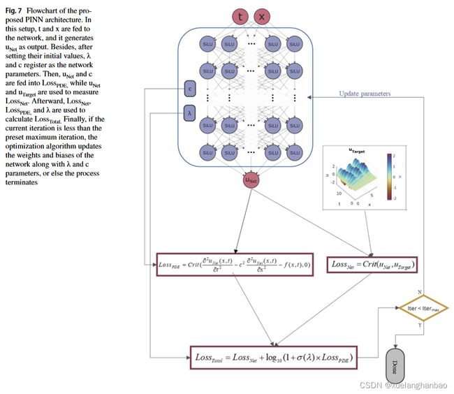
作者使用了解析解生成具有多个传播速度值( c = 8.0 、 4.0 、 2.0 、 1.0 、 0.5 m / s c = 8.0、4.0、2.0、1.0、0.5 m/s c=8.0、4.0、2.0、1.0、0.5m/s)的不同波浪模拟( 300 × 300 300 \times 300 300×300 的均匀网格),并从其中随机抽取4000个点作为已知数据,随后将其用作 PINN 的输入数据,用来识别传播速度 c c c。
其中,网络设置为由一个输入层、7 个中间(隐藏)层和一个输出层组成。每个中间层包含 25 个神经元。该架构采用 SiLU (Swish) 函数来激活中间层,并使用线性函数来激活输出层。 c c c 的初始值通过对真实值添加一个介于-1.0和1.0之间的随机值来设置。
该问题的损失函数如下:
L o s s T o t a l = L o s s N e t + λ L o s s P D E L o s s N e t = M S E ( u N e t , u T a r g e t ) L o s s P D E = M S E ( ∂ 2 u N e t ( x , t ) ∂ t 2 − c 2 ∂ 2 u N e t ( x , t ) ∂ x 2 , 0 ) \begin{aligned} &Loss_{Total}=Loss_{Net}+\lambda Loss_{PDE} \\ &Loss_{Net}=MSE(u_{Net},u_{Target}) \\ &Loss_{PDE}=MSE(\frac{\partial^{2}u_{Net}(x,t)}{\partial t^{2}}-c^{2}\frac{\partial^{2}u_{Net}(x,t)}{\partial x^{2}},0) \end{aligned} LossTotal=LossNet+λLossPDELossNet=MSE(uNet,uTarget)LossPDE=MSE(∂t2∂2uNet(x,t)−c2∂x2∂2uNet(x,t),0)
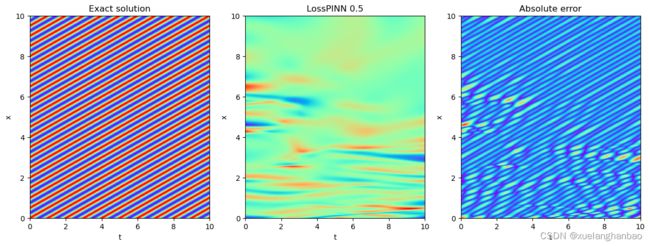
其中 u N e t u_{Net} uNet和 u T a r g e t u_{Target} uTarget 分别是网络的输出和目标波场。此设置使用均方误差 (MSE) 作为损失准则函数。此外, λ \lambda λ 是控制软PDE正则化对整个优化问题影响的乘数。该乘数的值应保持尽可能低,因为其较高的值会导致复杂的损失情况;通过反复试验,作者设置 λ = 0.1 \lambda = 0.1 λ=0.1。该设置通过均方误差计算损失,并且损失函数在这种情况下不考虑边界条件的单独项,因为该问题是一个具有无限边界的问题。为了确保结果的可比性,作者将相同的权重和偏差初始化加载到网络中。最后,进行了 6000 次 ADAM 迭代来训练网络。
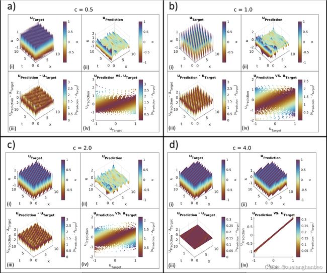
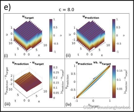
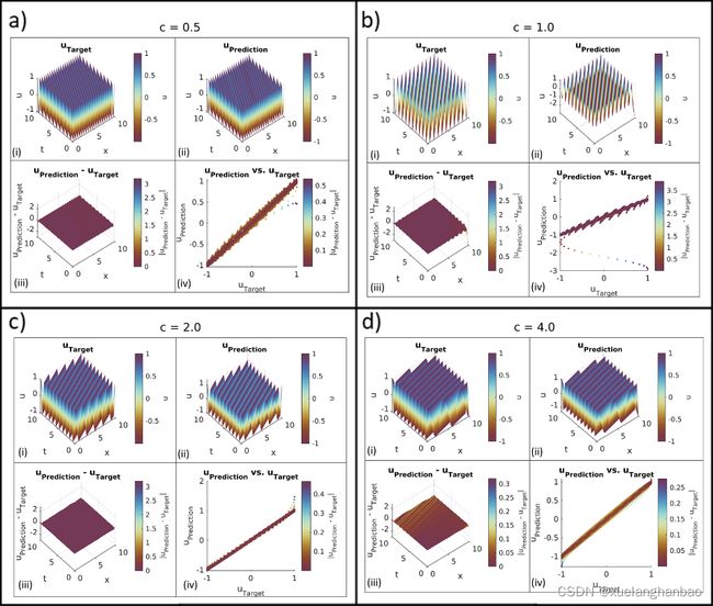
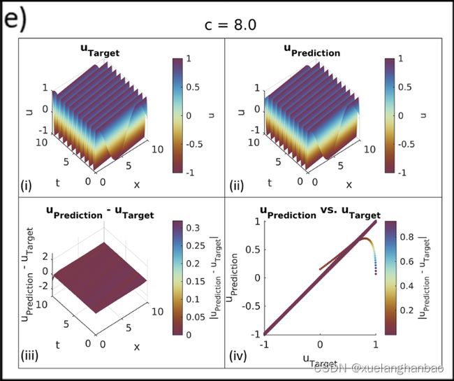
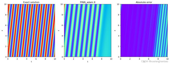
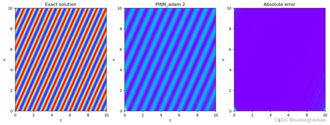
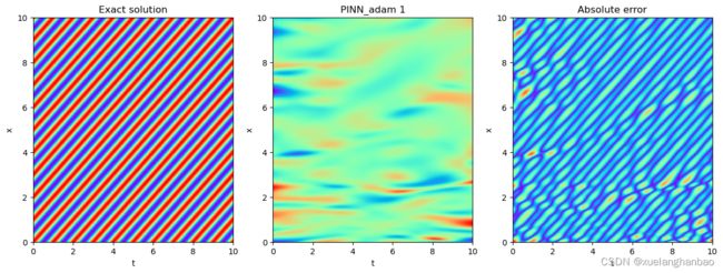
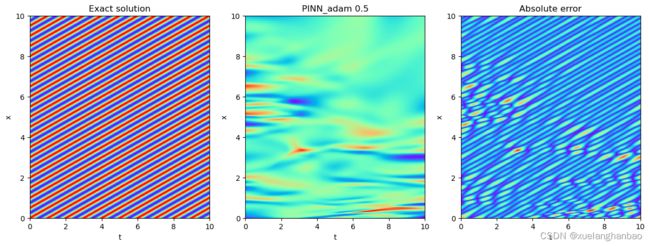
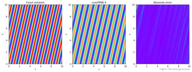
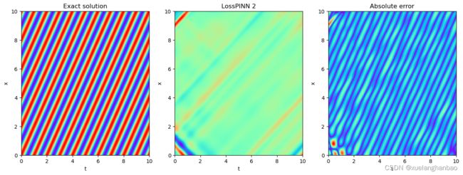
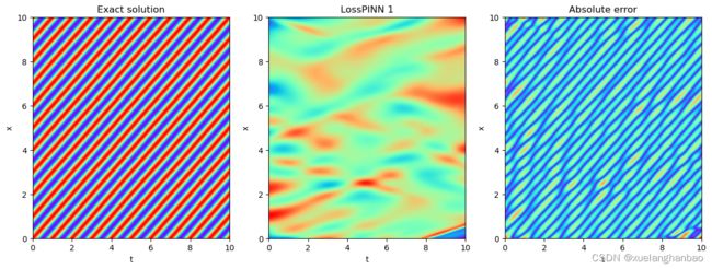
上图展示了普通 PINN 在该问题设置上的结果,
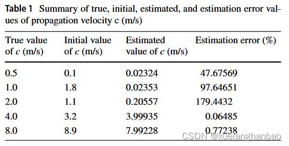
上表显示了 c 的初始猜测和估计值。该网络无法在 c = 0.5 、 1.0 c = 0.5、1.0 c=0.5、1.0 和 2.0 2.0 2.0 的情况下进行训练,这些情况具有更复杂的波场状态。这种失败可以从模型无法拟合波场 ( u u u) 和估计传播速度 ( c c c) 的不准确中观察到。
具有反射边界和源函数的情况
驻波是一个简单的例子。向问题引入反射边界、源函数和初始条件会产生更加复杂的解决方案。例如,考虑以下问题设置:
∂ 2 u ( x , t ) ∂ t 2 − c 2 ∂ 2 u ( x , t ) ∂ x 2 = f ( x , t ) , x ∈ ( 0 , 8 ) , t ∈ ( 0 , 16 ] c = 3.0 m / s f ( x , t ) = 100 × sin ( 4.0 × t ) × e − ( t − 7.0 ) 2 18.0 × e − ( x − 0.5 ) 2 0.02 , x ∈ ( 0 , 8 ) , t ∈ ( 0 , 16 ] u ( x , 0 ) = 0 , x ∈ [ 0 , 8 ] u ( 0 , t ) = 0 , t ∈ ( 0 , 16 ] u ( 8.0 , t ) = 0 , t ∈ ( 0 , 16 ] and L o s s T o t a l = L o s s N e t + λ L o s s P D E , L o s s N e t = M S E ( u N e t , u T a r g e t ) , L o s s P D E = M S E ( ∂ 2 u N e t ( x , t ) ∂ t 2 − c 2 ∂ 2 u N e t ( x , t ) ∂ x 2 − f ( x , t ) , 0 ) , \begin{aligned} &\frac{\partial^{2}u(x,t)}{\partial t^{2}}-c^{2}\frac{\partial^{2}u(x,t)}{\partial x^{2}}=f(x,t),& x\in(0,8),t\in(0,16] \\ &c=3.0\mathbf{m/s} \\ &f(x,t)=100\times\sin(4.0\times t)\times e^{-\frac{(t-7.0)^{2}}{18.0}}\times e^{-\frac{(x-0.5)^{2}}{0.02}},& x\in(0,8),t\in(0,16] \\ &u(x,0)=0,& x\in[0,8] \\ &u(0,t)=0,& t\in(0,16] \\ &u(8.0,t)=0,& t\in(0,16] \\ &\text{and} \\ &Loss_{Total}=Loss_{Net}+\lambda Loss_{PDE}, \\ &Loss_{Net}=MSE(u_{Net},u_{Target}), \\ &Loss_{PDE}=MSE(\frac{\partial^{2}u_{Net}(x,t)}{\partial t^{2}}-c^{2}\frac{\partial^{2}u_{Net}(x,t)}{\partial x^{2}}-f(x,t),0), \end{aligned} ∂t2∂2u(x,t)−c2∂x2∂2u(x,t)=f(x,t),c=3.0m/sf(x,t)=100×sin(4.0×t)×e−18.0(t−7.0)2×e−0.02(x−0.5)2,u(x,0)=0,u(0,t)=0,u(8.0,t)=0,andLossTotal=LossNet+λLossPDE,LossNet=MSE(uNet,uTarget),LossPDE=MSE(∂t2∂2uNet(x,t)−c2∂x2∂2uNet(x,t)−f(x,t),0),x∈(0,8),t∈(0,16]x∈(0,8),t∈(0,16]x∈[0,8]t∈(0,16]t∈(0,16]
作者使用有限差分方案生成了该问题的解集(在 x x x 和 t t t 的均匀网格上的 999 × 1000 999 \times 1000 999×1000 个 u u u 样本),然后对其进行二次采样( x 、 t x、t x、t 和 u u u 的 4000 个随机样本)以用于具有与上文相同架构的 PINN 设置
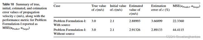
在此设置中, c c c 的目标值为 3.0 m / s 3.0 m/s 3.0m/s;作者将速度估计的起点设置为 2.1 m / s 2.1 m/s 2.1m/s,算法估计的速度等于 3.04557 m / s 3.04557 m/s 3.04557m/s。尽管该模型以较低的误差值估计了传播速度,但使用普通 PINN 预测的波场再次不令人满意,如下图所示:

分析
为了解决 PINN 的故障,作者分析了训练过程中 L o s s N e t 、 L o s s P D E Loss_{Net}、Loss_{PDE} LossNet、LossPDE 和 L o s s T o t a l Loss_{Total} LossTotal 值的趋势和模式。然后,作者将失败的案例与成功的案例进行比较,以确定训练过程中可能导致不同结果的任何差异。

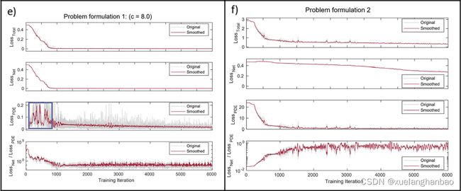
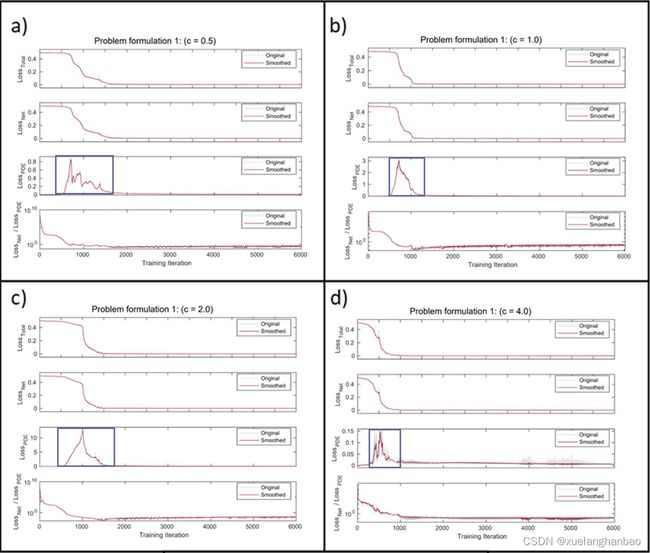
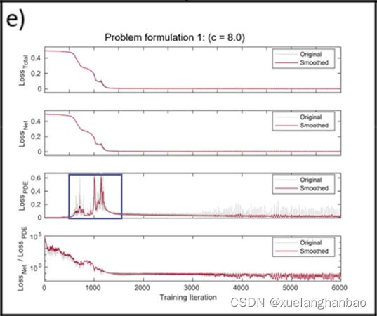
上图显示了每次迭代的问题损失值(即 L o s s N e t 、 L o s s P D E Loss_{Net}、Loss_{PDE} LossNet、LossPDE 和 L o s s T o t a l Loss_{Total} LossTotal )的曲线,
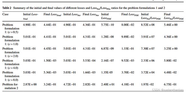
上表总结了每种情况的初始和最终损失。
在失败案例中( a 、 b 、 c 、 f a、b、c、f a、b、c、f), L o s s T o t a l Loss_{Total} LossTotal 在训练过程中并没有明显下降。另一方面,成功案例中 L o s s T o t a l Loss_{Total} LossTotal 则下降了多个数量级。对 L o s s N e t / L o s s P D E Loss_{Net}/Loss_{PDE} LossNet/LossPDE 比率和 L o s s P D E Loss_{PDE} LossPDE 曲线的分析揭示了两个临界点。首先,当 L o s s N e t / L o s s P D E Loss_{Net}/Loss_{PDE} LossNet/LossPDE 比率降至 1.0 1.0 1.0 以下时,训练过程就会成功(问题公式 2 除外,稍后讨论)。其次,当这些成功发生时, L o s s P D E Loss_{PDE} LossPDE 的衰减曲线显示出特定的上升和下降几何形状,在 d 、 e d、e d、e中使用方框突出显示。对各种案例的多重分析表明,这种行为与训练过程的成功密切相关。
可以通过训练过程观察生成的波场结构变化来理解这种现象。网络的随机权重和偏置初始化通常会生成一个波场 u u u,它可以满足波动方程的PDE,而无需与目标数据进行拟合(即低 L o s s P D E Loss_{PDE} LossPDE但高 L o s s N e t Loss_{Net} LossNet)。作者随机初始化了网络四次。然后,将 x x x 和 t t t 馈送到网络的这四个初始状态以生成波场 u u u。
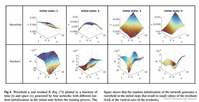
上图显示了具有不同初始化和残差 ® 的结果波场 u(问题 1公式: c = 2.0 c = 2.0 c=2.0)的图,残差根据以下方程计算:
∂ 2 u ( x , t ) ∂ t 2 − c 2 ∂ 2 u ( x , t ) ∂ x 2 = R ( x , t ) \frac{\partial^2u(x,t)}{\partial t^2}-c^2\frac{\partial^2u(x,t)}{\partial x^2}=R(x,t) ∂t2∂2u(x,t)−c2∂x2∂2u(x,t)=R(x,t)
从图中可以看出,这四种随机初始化的R值都是很小的,这表明随机初始化生成的波场能够较好地满足上述波动方程。
因此,在优化的初始迭代中, L o s s P D E Loss_{PDE} LossPDE 项较小。由于优化器在 L o s s T o t a l Loss_{Total} LossTotal 上工作, L o s s T o t a l Loss_{Total} LossTotal 是 L o s s N e t Loss_{Net} LossNet 和 L o s s P D E Loss_{PDE} LossPDE 的加权和,因此 L o s s P D E Loss_{PDE} LossPDE 小值导致优化器仅在 L o s s N e t Loss_{Net} LossNet 上工作。为了使 L o s s P D E Loss_{PDE} LossPDE 对 L o s s T o t a l Loss_{Total} LossTotal 做出更多贡献,从而调节优化问题,网络应首先使波场结构从其初始状态波动。这样做会导致 L o s s P D E Loss_{PDE} LossPDE 值增加,因此,这意味着优化器应该采取整体 L o s s T o t a l Loss_{Total} LossTotal 的上升路径。这种向上的路径不利于最小化算法,并且对寻找可接受的解决方案的过程造成了障碍。在不成功的情况下,训练算法并没有在初始步骤中经历 L o s s P D E Loss_{PDE} LossPDE 的急剧上升,然后利用正则化来寻找更好的解决方案,而是陷入了 L o s s N e t Loss_{Net} LossNet 的非常温和的局部最小值,在这个情况下,正则化再也无法帮助它。
损失景观的可视化可以显示故障模式下这种平缓的平台结构局部最小值。为了绘制损失图,作者使用 PyHessian 包沿着网络的训练参数其 Hessian 矩阵的第一和第二特征向量扰动网络参数,并计算每组扰动参数中的 L o s s N e t Loss_{Net} LossNet ,如下图所示:
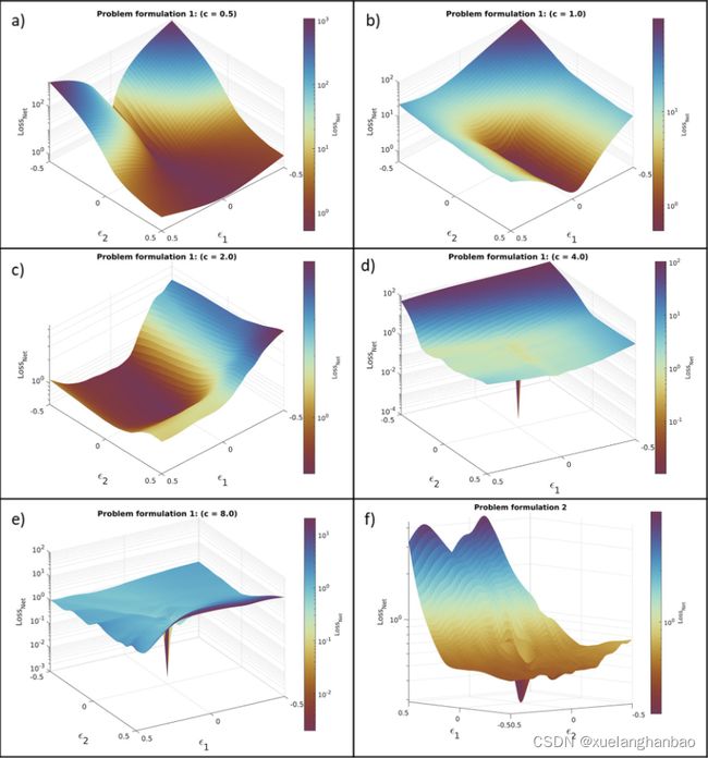
在 PINN 的成功案例中可以发现,损失函数沿最大特征向量方向的灵敏度最高,这会导致陡峭的最小值。损失景观的可视化显示,在故障情况下,这些突变并未沿着第一和第二特征向量的方向发生( a 、 b 、 c 、 f a、b、c、f a、b、c、f);相反,景观呈现出一种温和的结构。另一方面,在以下情况下 PINN 已经收敛( d 、 e d、e d、e),沿着 Hessian 矩阵的第一和第二特征向量的方向出现陡峭最小值。另一点需要提到的是,虽然问题 2 的损失的行为略有不同( L o s s N e t / L o s s P D E Loss_{Net}/Loss_{PDE} LossNet/LossPDE 的值低于 1.0,并且 L o s s P D E Loss_{PDE} LossPDE 的值没有明显上升),结果同样不令人满意。在这种情况下,训练达到了 L o s s P D E Loss_{PDE} LossPDE 下降的状态,因此它对优化的效果也下降了。因此, L o s s P D E Loss_{PDE} LossPDE 正则化无法对之后的整体问题做出进一步的贡献,并且问题陷入了局部最小值。
PINN 的普通设置的另一个问题是,它的收敛不仅受到解的复杂性的高度影响,而且还受到网络初始化和正则化乘数 λ \lambda λ 的值的影响。即使在最好的情况下(问题 1: c = 4.0 c = 4.0 c=4.0),不同初始化的许多立场或 λ \lambda λ 的轻微变化也可能导致失败,应该采用更稳健的方法来解决。
解决方法
对数PDE损失
在失效模式分析部分,作者表明 L o s s P D E Loss_{PDE} LossPDE 应先上升然后下降,以引导优化问题达到令人满意的最小值(即预测波场和目标波场拟合可接受的状态)。最小化算法(训练算法)将抵制 L o s s P D E Loss_{PDE} LossPDE 的增加(特别是对于更复杂的),因为它可能导致 L o s s T o t a l Loss_{Total} LossTotal 的增加。值小于 1 的正则化乘数 λ 的作用是让 L o s s P D E Loss_{PDE} LossPDE 能够自由地采取向上路径,而不会对 L o s s T o t a l Loss_{Total} LossTotal 产生很大的影响,但是,正如失败分析所示,这还不够。为 λ \lambda λ 分配较小的值也不合适,因为它会导致优化器在许多情况下不使用 L o s s P D E Loss_{PDE} LossPDE 项 。
因此,作者建议将 L o s s T o t a l Loss_{Total} LossTotal 更改如下:
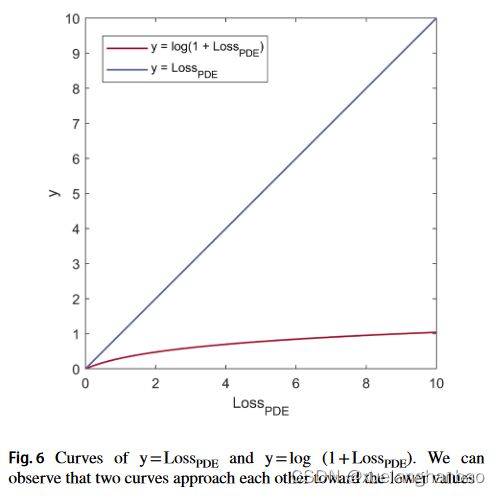
L o s s T o t a l = L o s s N e t + log ( 1 + L o s s P D E ) Loss_{Total}=Loss_{Net}+\log(1+Loss_{PDE}) LossTotal=LossNet+log(1+LossPDE)
由于这一修改, L o s s P D E Loss_{PDE} LossPDE 在训练过程的早期阶段有更多的自由度来采取向上的路径(不会因为正则化乘数的值较低而失去其效果)。
函数 log ( 1 + L o s s P D E ) \log(1+Loss_{PDE}) log(1+LossPDE) 的作用是通过降低 L o s s P D E Loss_{PDE} LossPDE 对 L o s s T o t a l Loss_{Total} LossTotal 的贡献来促进 L o s s P D E Loss_{PDE} LossPDE 的上升路径。另一方面,对于较低的值,函数 log ( 1 + L o s s P D E ) \log(1+Loss_{PDE}) log(1+LossPDE) 的结果接近 L o s s P D E Loss_{PDE} LossPDE 本身(如下图所示)。这种行为确保 L o s s P D E Loss_{PDE} LossPDE 即使变小时也不会失去其调节作用。
S形自适应正则化乘数 λ \lambda λ
λ \lambda λ 的值可以极大地控制问题的收敛性。一种方法是将这个量视为 PINN 结构的恒定超参数。然而,由于训练过程的收敛对 λ \lambda λ 参数很敏感,并且其最佳值可能因情况而异,因此手动设置该超参数可能会很麻烦。另一种方法是将 λ \lambda λ 增加到网络参数。因此,训练算法尝试在更新网络参数(即权重和偏差)的同时调整 λ \lambda λ 的最佳值。尽管第二种方法看起来很有希望,但它也有一些缺陷。首先,优化算法可能会导致负的 λ \lambda λ 值。其次,在许多情况下,这种方法会导致 λ \lambda λ 值极小,从而消除了 L o s s P D E Loss_{PDE} LossPDE 的正则化效果。为了解决这些问题,作者建议使用 λ \lambda λ 的 Sigmoid 作为正则化乘数。因此, L o s s T o t a l Loss_{Total} LossTotal 变为:
L o s s T o t a l = L o s s N e t + log ( 1 + σ ( λ ) × L o s s P D E ) Loss_{Total}=Loss_{Net}+\log(1+\sigma(\lambda)\times Loss_{PDE}) LossTotal=LossNet+log(1+σ(λ)×LossPDE)
其中 σ ( λ ) \sigma(\lambda) σ(λ) 是 λ \lambda λ 的 Sigmoid。这种方法具有多种好处。首先,Sigmoid 保证将在 L o s s P D E Loss_{PDE} LossPDE 中相乘的值低于1.0 且高于零。其次,Sigmoid 函数不会让 L o s s P D E Loss_{PDE} LossPDE 的乘数(即 σ ( λ ) \sigma(\lambda) σ(λ) )衰减得如此之快(因为 Sigmoid 函数的斜率变得平缓地趋向较小的值)。然而,作者考虑了 λ \lambda λ 的较低范围,以禁止 σ ( λ ) \sigma(\lambda) σ(λ) 取最小值,这可能会消除 PDE 正则化效应。当参数 λ \lambda λ 达到预设的下限时冻结其梯度,以防止其变小。
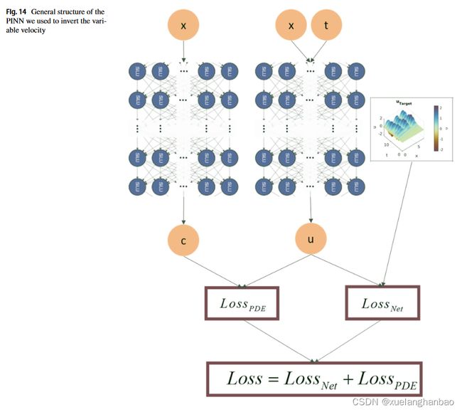
最后,本文提出的网络结构如下图所示:
实验结果
驻波
网络将 λ \lambda λ 和 c c c 视为参数,并通过训练过程更新它们。其中 λ \lambda λ 的初始值设置为10.0(因此, σ ( λ ) \sigma(\lambda) σ(λ) 近似等于1.0),并且每种情况下的传播速度 c c c 的值与先前所示的值相同。限制 λ \lambda λ 下限等于 − 4.6 − 4.6 −4.6 ,以防止 σ ( λ ) \sigma(\lambda) σ(λ) 变得小于 0.01。
上图表明该模型以可接受的精度预测了所有情况。
上图显示了训练过程中每个贡献损失的变化。对于所有这些情况, L o s s P D E Loss_{PDE} LossPDE 都遵循在初始步骤中从低值上升然后下降的行为,我们在普通 PINN 的成功案例中看到了这一点。它表明对数 L o s s P D E Loss_{PDE} LossPDE 已经被赋予了问题足够的自由度,达到了PDE正则化可以发挥作用的状态。在这种情况下,对数允许 L o s s P D E Loss_{PDE} LossPDE 上升到13.5,但它并没有迫使 L o s s T o t a l Loss_{Total} LossTotal 有明显的上升。此外,虽然 L o s s P D E Loss_{PDE} LossPDE 已经上升到了相对较高的值,但最终 L o s s N e t Loss_{Net} LossNet与 L o s s P D E Loss_{PDE} LossPDE 的比例已经下降到了一个数量级以下。
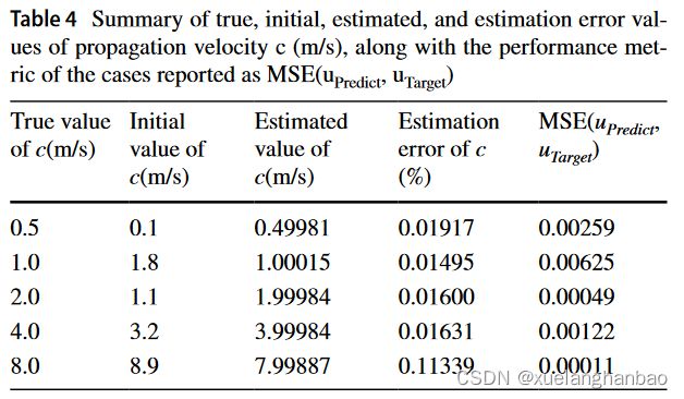
上表为对 c c c 的预测结果
具有反射边界和源函数的情况
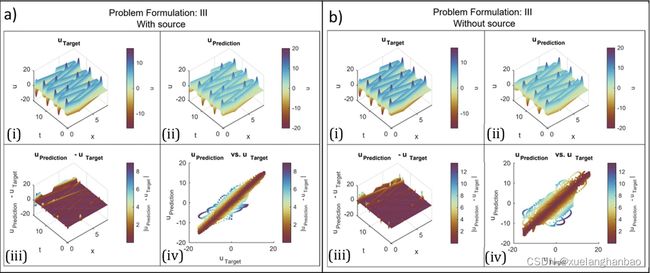
考虑和不考虑源函数
假设源函数未知。目的是研究即使在真正的基础物理未知的情况下,是否可以通过在修改后的 PINN 模型中实现最接近的可用物理来获得可接受的结果。为此,我们在 L o s s P D E Loss_{PDE} LossPDE 计算中忽略源项(即 f ( x , t ) f(x,t) f(x,t))并考虑波动方程的齐次形式。因此, L o s s P D E Loss_{PDE} LossPDE 计算如下:
L o s s P D E = C r i t ( ∂ 2 u N e t ( x , t ) ∂ t 2 − c 2 ∂ 2 u N e t ( x , t ) ∂ x 2 , 0 ) Loss_{PDE}=Crit(\frac{\partial^2u_{Net}(x,t)}{\partial t^2}-c^2\frac{\partial^2u_{Net}(x,t)}{\partial x^2},0) LossPDE=Crit(∂t2∂2uNet(x,t)−c2∂x2∂2uNet(x,t),0)
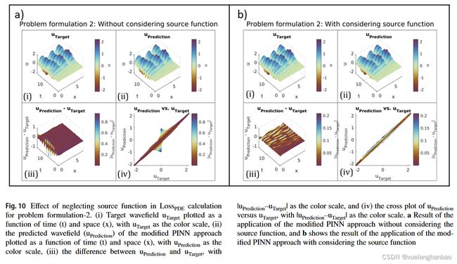
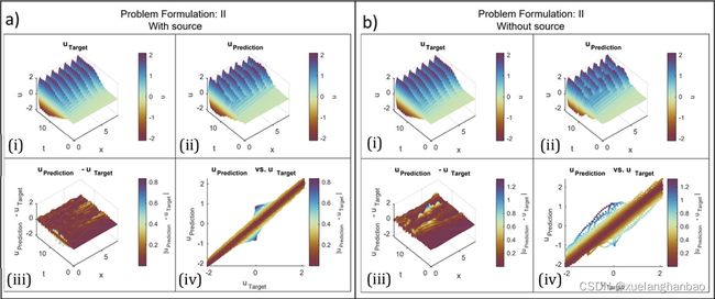
上图为两个结果的展示,比较这两个结果表明,虽然包含源函数可以预测更准确的结果,特别是在 x = 0.0 m x = 0.0 m x=0.0m 处的反射范围内,但不包含源函数的情况也得到了相对可接受的波场解和速度反演。这项检查表明,当缺乏有关源函数的信息时,忽略将其包含在方法的实现中是一个可行的选择。
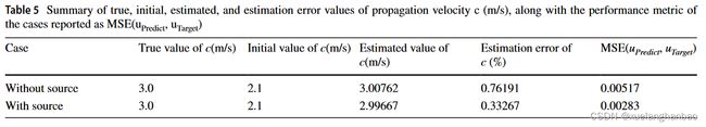
上表为最终 c c c 的估计值
损失标准评估
以往的研究工作中,PINN 架构中常用的损失准则是 MSE 和 MAE(平均绝对误差)。作者还测试了$ L^\infty$、LogCosh 和 Huber ,以检查哪一个显示出最佳性能。因此,为了比较不同标准的性能,作者设置了具有不同标准的模型
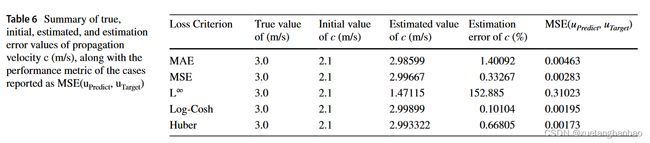
上表中提供了每个标准训练的模型的最终状态。
Is L 2 L^2 L2 Physics-Informed Loss Always Suitable for Training Physics-Informed Neural Network 已经表明 L ∞ L^\infty L∞ 在他们的情况下提供了最好的结果,但结果表明它在一维波动方程情况下表现不佳。基于 M S E ( u P r e d i c t , u T a r g e t ) MSE(u_{Predict}, u_{Target}) MSE(uPredict,uTarget),Huber提供了最好的性能,但是在Huber的情况下 c c c 的估计误差比在Log-Cosh的情况下更高。一般来说,这两种损失的性能都是可以接受的,因此作者在本研究的其余部分选择了 Huber 损失。
超参数调整
为了进一步增强模型,作者对模型应用了超参数调整。作者考虑了 L o s s B o u n d a r y Loss_{Boundary} LossBoundary 的单独项以及 L o s s N e t Loss_{Net} LossNet 和 L o s s B o u n d a r y Loss_{Boundary} LossBoundary 的常数乘数。因此, L o s s T o t a l Loss_{Total} LossTotal 变为:
L o s s T o t a l = α × L o s s N e t + β × L o s s B o u n d a r y + log ( 1 + σ ( λ ) × L o s s P D E ) Loss_{Total}=\alpha\times Loss_{Net}+\beta\times Loss_{Boundary}+\log(1+\sigma(\lambda)\times Loss_{PDE}) LossTotal=α×LossNet+β×LossBoundary+log(1+σ(λ)×LossPDE)
这里作者使用的是现成的参数搜索工具 Ray-Tune ,搜索了30个周期。
在本节的问题设置之前,作者已经得到了超参数调整的结果,并且前文已经应用了调整算法提出的通用网络结构。因此,在本节中,作者应用的修改是分离内部和边界搭配点损失(即 L o s s N e t Loss_{Net} LossNet 和 L o s s B o u n d a r y Loss_{Boundary} LossBoundary),并应用它们各自的乘数 α \alpha α 和 β \beta β 以及减小小批量大小。这两个修改稍微改善了结果。 M S E ( u P r e d i c t , u T a r g e t ) MSE(u_{Predict}, u_{Target}) MSE(uPredict,uTarget)下降至0.00066, c c c 的估计误差下降至 0.26193 0.26193% 0.26193 。
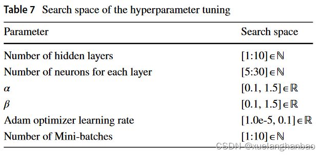
上表为参数的搜索空间。
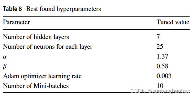
上表为得到的最优参数。
添加随机噪声
为了显示所提出的方法对噪声的鲁棒性,作者在目标数据(波场 u u u)上添加了三个级别的随机高斯白噪声(信噪比 S N R = 20 、 10 、 5 dB SNR= 20、10、5 \text{dB} SNR=20、10、5dB)。
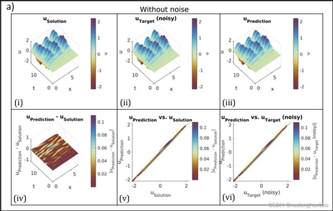
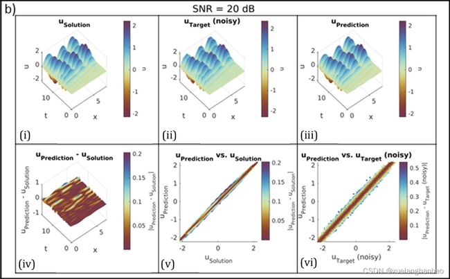


从上图可以看到,该模型在 S N R = 20 dB SNR = 20 \text{dB} SNR=20dB 和 10 dB 10 \text{dB} 10dB 的噪声情况下表现出可接受的性能,但在 S N R = 5 dB SNR = 5 \text{dB} SNR=5dB 的情况下,它失败了。然而,当在 S N R = 5 dB SNR = 5 \text{dB} SNR=5dB 的情况下向模型提供更多输入和目标数据样本(10000 个样本)时,模型取得了准确的结果。
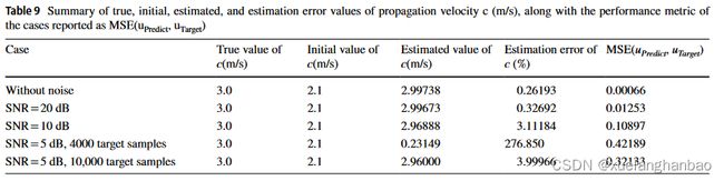
上表为不同噪声下对 c c c 预测的表现。
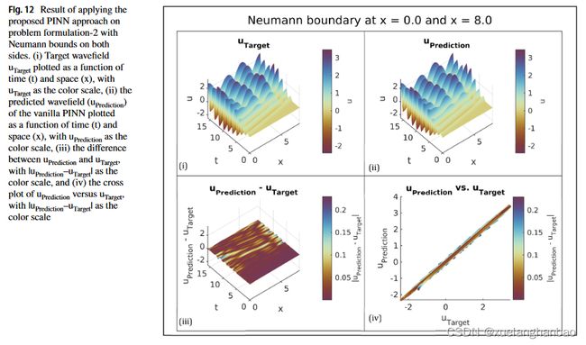
测试纽曼边界条件
考虑模型两侧的诺依曼边界条件,可以将其表述如下:
∂ 2 u ( x , t ) ∂ t 2 − c 2 ∂ 2 u ( x , t ) ∂ x 2 = f ( x , t ) . x ∈ ( 0 , 8 ) , t ∈ ( 0 , 16 ] c = 3.0 m / s f ( x , t ) = 100 × sin ( 4.0 × t ) × e − ( 4 − 7.00 ) 2 18.6 × e − ( x − 0.5 ) 2 0.60 , x ∈ ( 0 , 8 ) , t ∈ ( 0 , 16 ] u ( x , 0 ) = 0 , x ∈ [ 0 , 8 ] ∂ u ( 0 , t ) ∂ t = 0 , t ∈ ( 0 , 16 ] ∂ u ( 8.0 , t ) ∂ t = 0 , t ∈ ( 0 , 16 ] \begin{aligned} &\frac{\partial^{2}u(x,t)}{\partial t^{2}}-c^{2}\frac{\partial^{2}u(x,t)}{\partial x^{2}}=f(x,t)& \text{.} &&&& x\in(0,8),t\in(0,16] \\ &c=3.0\mathrm{m/s} \\ &f(x,t)=100\times\sin(4.0\times t)\times e^{-{\frac{(4-7.00)^{2}}{18.6}}}\times e^{-{\frac{(x-0.5)^{2}}{0.60}}},&&& x\in(0,8),t\in(0,16] \\ &u(x,0)=0,&&& x\in[0,8] \\ &\frac{\partial u(0,t)}{\partial t}=0,&&& t\in(0,16] \\ &\frac{\partial u(8.0,t)}{\partial t}=0,&&& t\in(0,16] \end{aligned} ∂t2∂2u(x,t)−c2∂x2∂2u(x,t)=f(x,t)c=3.0m/sf(x,t)=100×sin(4.0×t)×e−18.6(4−7.00)2×e−0.60(x−0.5)2,u(x,0)=0,∂t∂u(0,t)=0,∂t∂u(8.0,t)=0,.x∈(0,8),t∈(0,16]x∈[0,8]t∈(0,16]t∈(0,16]x∈(0,8),t∈(0,16]
同样采用有限差分方案来生成包含 999 × 1000 999\times 1000 999×1000 个 u u u 样本的解集,均匀分布在 x x x 和 t t t 维度上。随后,对该数据集进行二次采样,以获得 x 、 t x、t x、t 和 u u u 的 4000 个随机样本,这些样本用作通过超参数调整确定的 PINN 配置的输入。从初始值 c = 2.1 m / s c = 2.1 m/s c=2.1m/s 开始,最终模型估计速度为 3.00132 m / s 3.00132 m/s 3.00132m/s,估计误差仅为 0.13239 % 0.13239\% 0.13239%,结果如下图所示:
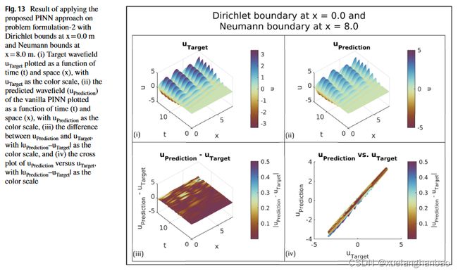
接下来,作者制定了一个问题配置,其中边界的一侧表现出狄利克雷边界条件,而另一侧表现出诺依曼边界条件。该设置可以描述如下:
∂ 2 u ( x , t ) ∂ t 2 − c 2 ∂ 2 u ( x , t ) ∂ x 2 = f ( x , t ) , x ∈ ( 0 , 8 ) , t ∈ ( 0 , 16 ] c = 3.0 m / s f ( x , t ) = 100 × sin ( 4.0 × t ) × e − ( t − 70 ) 2 180 × e − ( x − 0.5 ) 2 0.02 , x ∈ ( 0 , 8 ) , t ∈ ( 0 , 16] u ( x , 0 ) = 0 , x ∈ [ 0 , 8 ] u ( 0 , t ) = 0 , t ∈ ( 0 , 16 ] ∂ u ( 8.0 , t ) ∂ t = 0 , t ∈ ( 0 , 16 ] \begin{aligned} &\frac{\partial^{2}u(x,t)}{\partial t^{2}}-c^{2}\frac{\partial^{2}u(x,t)}{\partial x^{2}}=f(x,t),& x\in(0,8),t\in(0,16] \\ &c=3.0\mathrm{m/s} \\ &f(x,t)=100\times\sin(4.0\times t)\times e^{-\frac{(t-70)^{2}}{180}}\times e^{-\frac{(x-0.5)^{2}}{0.02}},\quad &x\in(0,8),t\in(0,\text{16]} \\ &u(x,0)=0,& x\in[0,8] \\ &u(0,t)=0,& t\in(0,16] \\ &\frac{\partial u(8.0,t)}{\partial t} =0, & t\in(0,16] \end{aligned} ∂t2∂2u(x,t)−c2∂x2∂2u(x,t)=f(x,t),c=3.0m/sf(x,t)=100×sin(4.0×t)×e−180(t−70)2×e−0.02(x−0.5)2,u(x,0)=0,u(0,t)=0,∂t∂u(8.0,t)=0,x∈(0,8),t∈(0,16]x∈(0,8),t∈(0,16]x∈[0,8]t∈(0,16]t∈(0,16]
最终模型估计速度等于 2.99347 m/s,导致估计误差为 0.65305%,结果如下图所示:
变速情况
考虑如下变速问题:
$$
\begin{aligned}
&\frac{\partial^2u(x,t)}{\partial t^{2}}{\partial t^{2}}-\frac{\partial}{\partial x}(c^{2}(x)\frac{\partial u(x,t)}{\partial x})=0, &x\in(0,8),t\in(0,16] \
&c(x)=\left{\begin{array}
{ll}{0.6\mathrm{m/s},x\leq1.2}\
{0.4\mathrm{m/s},1.2
&u(x,0)=e{(-0.5\times({\frac{x-0.5}{0.1}}){2})},& x\in[0,8] \
&u(0,t)=0,& t\in(0,16] \
&u(8.0,t)=0,& \iota\in(0,16] \
&\text{and} \
&Loss_{Total}=Loss_{Net}+\lambda Loss_{PDE}, \
&Ioss_{Net}=MSE(u_{Net},u_{Target}), \
&Loss_{PDE}=MSE(\frac{\partial^{2}u_{Net}(x,t)}{\partial t^{2}}-\frac{\partial}{\partial x}(c^{2}(x)\frac{\partial u_{Net}(x,t)}{\partial x}),0),
\end{aligned}
$$
此时,网络结构如下:

上图为训练结果展示。
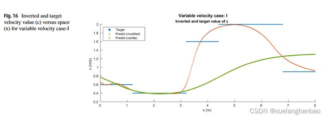
上图为对 c c c 的预测结果展示
不同源函数情况
考虑振幅更高的源函数:
f ( x , t ) = 10000 × sin ( 4.0 × t ) × e − ( t − 7.0 ) 2 18.0 × e − ( x − 0.5 ) 2 0.02 , x ∈ ( 0 , 8 ) , t ∈ ( 0 , 16 ] f(x,t)=10000\times\sin(4.0\times t)\times e^{-\frac{(t-7.0)^2}{18.0}}\times e^{-\frac{(x-0.5)^2}{0.02}},\quad x\in(0,8),t\in(0,16] f(x,t)=10000×sin(4.0×t)×e−18.0(t−7.0)2×e−0.02(x−0.5)2,x∈(0,8),t∈(0,16]

考虑更震荡的源函数:
f ( x , t ) = 100 × sin ( 8.0 × t ) × e − ( t − 7.0 ) 2 18.0 × e − ( x − 0.5 ) 2 0.02 , x ∈ ( 0 , 8 ) , t ∈ ( 0 , 16 ] f(x,t)=100\times\sin(8.0\times t)\times e^{-\frac{(t-7.0)^2}{18.0}}\times e^{-\frac{(x-0.5)^2}{0.02}},x\in(0,8),\mathrm{~}t\in(0,16] f(x,t)=100×sin(8.0×t)×e−18.0(t−7.0)2×e−0.02(x−0.5)2,x∈(0,8), t∈(0,16]

考虑其能量在相对较短的时间内释放的情况:
f ( x , t ) = 3000 × ( 1 − 200 × π 2 × ( t − 0.5 ) 2 ) × e − 200 × x 2 × ( t − 0.5 ) 2 × e − ( x − 2.5 ) 2 0.02 , x ∈ ( 0 , 8 ) , t ∈ ( 0 , 16 ] f(x,t)=3000\times(1-200\times\pi^{2}\times(t-0.5)^{2})\times e^{-200\times x^{2}\times(t-0.5)^{2}}\times e^{-\frac{(x-2.5)^{2}}{0.02}},x\in(0,8),t\in(0,16] f(x,t)=3000×(1−200×π2×(t−0.5)2)×e−200×x2×(t−0.5)2×e−0.02(x−2.5)2,x∈(0,8),t∈(0,16]

总结
本文以一维波动方程为例,对PINN训练过程中的损失下降情况进行了实验观察,发现训练成功的样例中PDE损失项都出现了先上升再下降的现象。随后作者提出,应当在PINN训练早期减少对PDE损失项的敏感度,于是作者使用 log \log log函数以及经过 σ \sigma σ 归一化的动态权重 λ \lambda λ 来实现了这一想法,并在多个不同样例上取得了显著的改善。
在训练前期需要注重真实数据的损失这一点个人是非常认同的,但对于使用 log ( 1 + σ ( λ ) L o s s P D E ) \log(1+\sigma(\lambda)Loss_{PDE}) log(1+σ(λ)LossPDE) 这样的形式似乎还不是很完善。看了一下作者提到的自适应权重那篇文章,从结果来看,其实就是把权重设置为可训练,然后损失项里添加了一个正则化项,让权重不会太小。本文里作者没有添加正则化项,但是对 σ ( λ ) \sigma(\lambda) σ(λ) 进行了截断,考虑到最优情况下权重肯定是越小越好,因此猜测 σ ( λ ) \sigma(\lambda) σ(λ) 最终就是设置的截断值 0.01 0.01 0.01 ,因此,后期这个方法相当于是在权重 log ( 1 + 0.01 ) = 0.095 \log(1+0.01)=0.095 log(1+0.01)=0.095 的情况下进行训练?作者没有提供代码,目前我复现的代码并没有文中那么好的结果。
PINN结果:

本文方法结果:

相关链接:
- 原文:Manipulating the loss calculation to enhance the training process of physics-informed neural networks to solve the 1D wave equation | SpringerLink
- 个人复现代码:Manipulating the loss calculation to enhance the training process of physics-informed neural networks to solve the 1D wave equation: Manipulating the loss calculation to enhance the training process of physics-informed neural networks to solve the 1D wave equation (gitee.com)