深度学习 Day14——P3天气识别

• 本文为365天深度学习训练营 中的学习记录博客
• 原作者：K同学啊 | 接辅导、项目定制

---

前言

本文将采用pytorch框架创建CNN网络，实现天气识别。讲述实现代码与执行结果，并浅谈涉及知识点。
关键字： torchvision.transforms.Compose()详解,pathlib中glob匹配多个格式文件获取数据列表,plt.tight_layout()作用,x.view()函数，The freeze_support error解决方案，提升测试acc–改变优化器。

1 我的环境

• 电脑系统：Windows 11
• 语言环境：python 3.8.6
• 编译器：pycharm2020.2.3
• 深度学习环境：
  torch == 1.9.1+cu111
  torchvision == 0.10.1+cu111
• 显卡：NVIDIA GeForce RTX 4070

2 代码实现与执行结果

2.1 前期准备

2.1.1 引入库

import torch
import torch.nn as nn

from torchvision import transforms, datasets
import os
from pathlib import Path
from PIL import Image
from torchinfo import summary
import torch.nn.functional as F
import matplotlib.pyplot as plt

plt.rcParams['font.sans-serif'] = ['SimHei']  # 用来正常显示中文标签
plt.rcParams['axes.unicode_minus'] = False  # 用来正常显示负号
plt.rcParams['figure.dpi'] = 100  # 分辨率
import warnings

warnings.filterwarnings('ignore')  # 忽略一些warning内容，无需打印

2.1.2 设置GPU（如果设备上支持GPU就使用GPU,否则使用CPU）

"""前期准备-设置GPU"""
# 如果设备上支持GPU就使用GPU,否则使用CPU
 device = torch.device("cuda" if torch.cuda.is_available() else "cpu")
 print("Using {} device".format(device))

输出

Using cuda device

2.1.3 导入数据

'''前期工作-导入数据'''
data_dir = "D:/DeepLearning/data/weather_photos/"
data_dir = Path(data_dir)

data_paths = list(data_dir.glob('*'))
classeNames = [str(path).split("\\")[-1] for path in data_paths]
print(classeNames)

输出

['cloudy', 'rain', 'shine', 'sunrise']

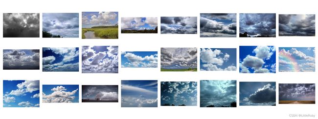
2.1.4 可视化数据

'''前期工作-可视化数据'''
# 指定图像文件夹路径
image_folder = os.path.join(data_dir, 'cloudy/')
# 获取文件夹中的所有图像文件
image_files = [f for f in os.listdir(image_folder) if f.endswith((".jpg", ".png", ".jpeg"))]
# 创建Matplotlib图像
fig, axes = plt.subplots(3, 8, figsize=(16, 6))
# 使用列表推导式加载和显示图像
for ax, img_file in zip(axes.flat, image_files):
    img_path = os.path.join(image_folder, img_file)
    img = Image.open(img_path)
    ax.imshow(img)
    ax.axis('off')
# 显示图像
plt.tight_layout()
plt.show()

2.1.4 图像数据变换

'''前期工作-图像数据变换'''
total_datadir = data_dir

# 关于transforms.Compose的更多介绍可以参考：https://blog.csdn.net/qq_38251616/article/details/124878863
train_transforms = transforms.Compose([
    transforms.Resize([224, 224]),  # 将输入图片resize成统一尺寸
    transforms.ToTensor(),  # 将PIL Image或numpy.ndarray转换为tensor，并归一化到[0,1]之间
    transforms.Normalize(  # 标准化处理-->转换为标准正太分布（高斯分布），使模型更容易收敛
        mean=[0.485, 0.456, 0.406],
        std=[0.229, 0.224, 0.225])  # 其中 mean=[0.485,0.456,0.406]与std=[0.229,0.224,0.225] 从数据集中随机抽样计算得到的。
])
total_data = datasets.ImageFolder(total_datadir, transform=train_transforms)
print(total_data)

输出

Dataset ImageFolder
    Number of datapoints: 1125
    Root location: D:\DeepLearning\data\weather_photos
    StandardTransform
Transform: Compose(
               Resize(size=[224, 224], interpolation=bilinear, max_size=None, antialias=None)
               ToTensor()
               Normalize(mean=[0.485, 0.456, 0.406], std=[0.229, 0.224, 0.225])
           )

2.1.4 划分数据集

'''前期工作-划分数据集'''
train_size = int(0.8 * len(total_data))  # train_size表示训练集大小，通过将总体数据长度的80%转换为整数得到；
test_size = len(total_data) - train_size  # test_size表示测试集大小，是总体数据长度减去训练集大小。
# 使用torch.utils.data.random_split()方法进行数据集划分。该方法将总体数据total_data按照指定的大小比例（[train_size, test_size]）随机划分为训练集和测试集，
# 并将划分结果分别赋值给train_dataset和test_dataset两个变量。
train_dataset, test_dataset = torch.utils.data.random_split(total_data, [train_size, test_size])
print(train_dataset, test_dataset)

输出

2.1.4 加载数据

'''前期工作-加载数据'''
batch_size = 32

train_dl = torch.utils.data.DataLoader(train_dataset,
                                       batch_size=batch_size,
                                       shuffle=True,
                                       num_workers=1)
test_dl = torch.utils.data.DataLoader(test_dataset,
                                      batch_size=batch_size,
                                      shuffle=True,
                                      num_workers=1)

2.1.4 查看数据

'''前期工作-查看数据'''
for X, y in test_dl:
    print("Shape of X [N, C, H, W]: ", X.shape)
    print("Shape of y: ", y.shape, y.dtype)
    break

输出

Shape of X [N, C, H, W]:  torch.Size([32, 3, 224, 224])
Shape of y:  torch.Size([32]) torch.int64

2.2 构建CNN网络模型

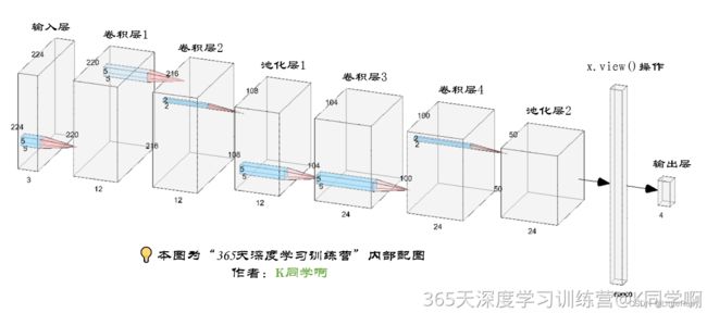
"""构建CNN网络"""
class Network_bn(nn.Module):
    def __init__(self):
        super(Network_bn, self).__init__()
        """
        nn.Conv2d()函数：
        第一个参数（in_channels）是输入的channel数量
        第二个参数（out_channels）是输出的channel数量
        第三个参数（kernel_size）是卷积核大小
        第四个参数（stride）是步长，默认为1
        第五个参数（padding）是填充大小，默认为0
        """
        self.conv1 = nn.Conv2d(in_channels=3, out_channels=12, kernel_size=5, stride=1, padding=0)
        self.bn1 = nn.BatchNorm2d(12)
        self.conv2 = nn.Conv2d(in_channels=12, out_channels=12, kernel_size=5, stride=1, padding=0)
        self.bn2 = nn.BatchNorm2d(12)
        self.pool = nn.MaxPool2d(2, 2)
        self.conv4 = nn.Conv2d(in_channels=12, out_channels=24, kernel_size=5, stride=1, padding=0)
        self.bn4 = nn.BatchNorm2d(24)
        self.conv5 = nn.Conv2d(in_channels=24, out_channels=24, kernel_size=5, stride=1, padding=0)
        self.bn5 = nn.BatchNorm2d(24)
        self.fc1 = nn.Linear(24 * 50 * 50, len(classeNames))

    def forward(self, x):
        x = F.relu(self.bn1(self.conv1(x)))
        x = F.relu(self.bn2(self.conv2(x)))
        x = self.pool(x)
        x = F.relu(self.bn4(self.conv4(x)))
        x = F.relu(self.bn5(self.conv5(x)))
        x = self.pool(x)
        x = x.view(-1, 24 * 50 * 50)
        x = self.fc1(x)

        return x
        
model = Network_bn().to(device)
print(model)
summary(model)        

输出

Network_bn(
  (conv1): Conv2d(3, 12, kernel_size=(5, 5), stride=(1, 1))
  (bn1): BatchNorm2d(12, eps=1e-05, momentum=0.1, affine=True, track_running_stats=True)
  (conv2): Conv2d(12, 12, kernel_size=(5, 5), stride=(1, 1))
  (bn2): BatchNorm2d(12, eps=1e-05, momentum=0.1, affine=True, track_running_stats=True)
  (pool): MaxPool2d(kernel_size=2, stride=2, padding=0, dilation=1, ceil_mode=False)
  (conv4): Conv2d(12, 24, kernel_size=(5, 5), stride=(1, 1))
  (bn4): BatchNorm2d(24, eps=1e-05, momentum=0.1, affine=True, track_running_stats=True)
  (conv5): Conv2d(24, 24, kernel_size=(5, 5), stride=(1, 1))
  (bn5): BatchNorm2d(24, eps=1e-05, momentum=0.1, affine=True, track_running_stats=True)
  (fc1): Linear(in_features=60000, out_features=4, bias=True)
)
=================================================================
Layer (type:depth-idx)                   Param #
=================================================================
Network_bn                               --
├─Conv2d: 1-1                            912
├─BatchNorm2d: 1-2                       24
├─Conv2d: 1-3                            3,612
├─BatchNorm2d: 1-4                       24
├─MaxPool2d: 1-5                         --
├─Conv2d: 1-6                            7,224
├─BatchNorm2d: 1-7                       48
├─Conv2d: 1-8                            14,424
├─BatchNorm2d: 1-9                       48
├─Linear: 1-10                           240,004
=================================================================
Total params: 266,320
Trainable params: 266,320
Non-trainable params: 0
=================================================================

2.3 训练模型

2.3.1 训练模型

"""训练模型--设置超参数"""
loss_fn = nn.CrossEntropyLoss()  # 创建损失函数，计算实际输出和真实相差多少，交叉熵损失函数，事实上，它就是做图片分类任务时常用的损失函数
learn_rate = 1e-4  # 学习率
opt = torch.optim.SGD(model.parameters(), lr=learn_rate)  # 作用是定义优化器，用来训练时候优化模型参数；其中，SGD表示随机梯度下降，用于控制实际输出y与真实y之间的相差有多大

2.3.2 编写训练函数

"""训练模型--编写训练函数"""
# 训练循环
def train(dataloader, model, loss_fn, optimizer):
    size = len(dataloader.dataset)  # 训练集的大小，一共60000张图片
    num_batches = len(dataloader)  # 批次数目，1875（60000/32）

    train_loss, train_acc = 0, 0  # 初始化训练损失和正确率

    for X, y in dataloader:  # 加载数据加载器，得到里面的 X（图片数据）和 y（真实标签）
        X, y = X.to(device), y.to(device) # 用于将数据存到显卡

        # 计算预测误差
        pred = model(X)  # 网络输出
        loss = loss_fn(pred, y)  # 计算网络输出和真实值之间的差距，targets为真实值，计算二者差值即为损失

        # 反向传播
        optimizer.zero_grad()  # 清空过往梯度
        loss.backward()  # 反向传播，计算当前梯度
        optimizer.step()  # 根据梯度更新网络参数

        # 记录acc与loss
        train_acc += (pred.argmax(1) == y).type(torch.float).sum().item()
        train_loss += loss.item()

    train_acc /= size
    train_loss /= num_batches

    return train_acc, train_loss

2.3.3 编写测试函数

"""训练模型--编写测试函数"""
# 测试函数和训练函数大致相同，但是由于不进行梯度下降对网络权重进行更新，所以不需要传入优化器
def test(dataloader, model, loss_fn):
    size = len(dataloader.dataset)  # 测试集的大小，一共10000张图片
    num_batches = len(dataloader)  # 批次数目，313（10000/32=312.5，向上取整）
    test_loss, test_acc = 0, 0

    # 当不进行训练时，停止梯度更新，节省计算内存消耗
    with torch.no_grad(): # 测试时模型参数不用更新，所以 no_grad，整个模型参数正向推就ok，不反向更新参数
        for imgs, target in dataloader:
            imgs, target = imgs.to(device), target.to(device)

            # 计算loss
            target_pred = model(imgs)
            loss = loss_fn(target_pred, target)

            test_loss += loss.item()
            test_acc += (target_pred.argmax(1) == target).type(torch.float).sum().item()#统计预测正确的个数

    test_acc /= size
    test_loss /= num_batches

    return test_acc, test_loss

2.3.4 正式训练

"""训练模型--正式训练"""
epochs = 20
train_loss = []
train_acc = []
test_loss = []
test_acc = []

for epoch in range(epochs):
    model.train()
    epoch_train_acc, epoch_train_loss = train(train_dl, model, loss_fn, opt)

    model.eval()
    epoch_test_acc, epoch_test_loss = test(test_dl, model, loss_fn)

    train_acc.append(epoch_train_acc)
    train_loss.append(epoch_train_loss)
    test_acc.append(epoch_test_acc)
    test_loss.append(epoch_test_loss)

    template = ('Epoch:{:2d}, Train_acc:{:.1f}%, Train_loss:{:.3f}, Test_acc:{:.1f}%，Test_loss:{:.3f}')
    print(template.format(epoch + 1, epoch_train_acc * 100, epoch_train_loss, epoch_test_acc * 100, epoch_test_loss))
print('Done')

输出

Epoch: 1, Train_acc:55.8%, Train_loss:1.098, Test_acc:58.7%，Test_loss:1.073
Epoch: 2, Train_acc:79.8%, Train_loss:0.682, Test_acc:74.2%，Test_loss:1.073
Epoch: 3, Train_acc:83.7%, Train_loss:0.536, Test_acc:78.2%，Test_loss:0.552
Epoch: 4, Train_acc:85.3%, Train_loss:0.472, Test_acc:80.9%，Test_loss:0.466
Epoch: 5, Train_acc:88.4%, Train_loss:0.412, Test_acc:82.7%，Test_loss:0.477
Epoch: 6, Train_acc:88.8%, Train_loss:0.367, Test_acc:88.0%，Test_loss:0.418
Epoch: 7, Train_acc:90.7%, Train_loss:0.318, Test_acc:88.4%，Test_loss:0.411
Epoch: 8, Train_acc:91.4%, Train_loss:0.288, Test_acc:86.2%，Test_loss:0.371
Epoch: 9, Train_acc:91.8%, Train_loss:0.289, Test_acc:86.7%，Test_loss:0.377
Epoch:10, Train_acc:91.4%, Train_loss:0.282, Test_acc:89.3%，Test_loss:0.342
Epoch:11, Train_acc:93.1%, Train_loss:0.248, Test_acc:89.3%，Test_loss:0.332
Epoch:12, Train_acc:93.6%, Train_loss:0.230, Test_acc:87.6%，Test_loss:0.344
Epoch:13, Train_acc:94.8%, Train_loss:0.216, Test_acc:88.9%，Test_loss:0.381
Epoch:14, Train_acc:94.2%, Train_loss:0.206, Test_acc:87.6%，Test_loss:0.340
Epoch:15, Train_acc:94.8%, Train_loss:0.199, Test_acc:88.4%，Test_loss:0.316
Epoch:16, Train_acc:94.7%, Train_loss:0.205, Test_acc:88.4%，Test_loss:0.475
Epoch:17, Train_acc:95.7%, Train_loss:0.222, Test_acc:86.7%，Test_loss:0.340
Epoch:18, Train_acc:96.1%, Train_loss:0.200, Test_acc:88.0%，Test_loss:0.319
Epoch:19, Train_acc:95.4%, Train_loss:0.182, Test_acc:88.4%，Test_loss:0.337
Epoch:20, Train_acc:96.8%, Train_loss:0.192, Test_acc:89.3%，Test_loss:0.304
Done

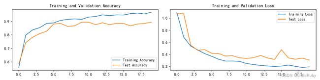
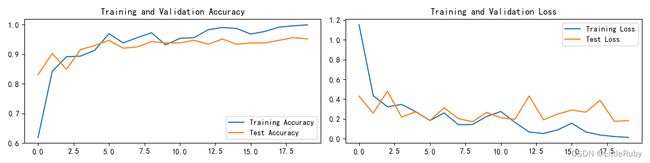
2.4 结果可视化

"""训练模型--结果可视化"""
epochs_range = range(epochs)

plt.figure(figsize=(12, 3))
plt.subplot(1, 2, 1)

plt.plot(epochs_range, train_acc, label='Training Accuracy')
plt.plot(epochs_range, test_acc, label='Test Accuracy')
plt.legend(loc='lower right')
plt.title('Training and Validation Accuracy')

plt.subplot(1, 2, 2)
plt.plot(epochs_range, train_loss, label='Training Loss')
plt.plot(epochs_range, test_loss, label='Test Loss')
plt.legend(loc='upper right')
plt.title('Training and Validation Loss')
plt.show()

3 知识点详解

3.1 torchvision.transforms.Compose()详解

torchvision是pytorch的一个图形库，它服务于PyTorch深度学习框架的，主要用来构建计算机视觉模型。torchvision.transforms主要是用于常见的一些图形变换。以下是torchvision的构成：

1.torchvision.datasets: 一些加载数据的函数及常用的数据集接口；
2.torchvision.models: 包含常用的模型结构（含预训练模型），例如AlexNet、VGG、ResNet等；
3.torchvision.transforms: 常用的图片变换，例如裁剪、旋转等；
4.torchvision.utils: 其他的一些有用的方法。

torchvision.transforms.Compose()类的主要作用是串联多个图片变换的操作。

from torchvision.transforms import transforms

train_transforms = transforms.Compose([
    transforms.Resize([224, 224]),                  # 将输入图片resize成统一尺寸
    transforms.RandomRotation(degrees=(-10, 10)),   # 随机旋转，-10到10度之间随机选
    transforms.RandomHorizontalFlip(p=0.5),         # 随机水平翻转 选择一个概率概率
    transforms.RandomVerticalFlip(p=0.5),           # 随机垂直翻转
    transforms.RandomPerspective(distortion_scale=0.6, p=1.0),    # 随机视角
    transforms.GaussianBlur(kernel_size=(5, 9), sigma=(0.1, 5)),  # 随机选择的高斯模糊模糊图像
    transforms.ToTensor(),          # 将PIL Image或numpy.ndarray转换为tensor，并归一化到[0,1]之间
    transforms.Normalize(           # 标准化处理-->转换为标准正太分布（高斯分布），使模型更容易收敛
        mean=[0.485, 0.456, 0.406], 
        std = [0.229, 0.224, 0.225])  # 其中 mean=[0.485,0.456,0.406]与std=[0.229,0.224,0.225] 从数据集中随机抽样计算得到的。
])

参考链接:torchvision.transforms.Compose()详解【Pytorch入门手册】

3.2 pathlib中glob匹配多个格式文件获取数据列表

可视化数据可用另一种方式显示

'''数据预处理-可视化数据'''
    cloudyPath = Path(data_dir)/"cloudy"
    image_files = list(p.resolve() for p in cloudyPath.glob('*') if p.suffix in [".jpg", ".png", ".jpeg"])

    plt.figure(figsize=(16, 6))
    for i in range(len(image_files[:24])):
        image_file = image_files[i]
        ax = plt.subplot(3, 8, i + 1)
        img = Image.open(str(image_file))
        plt.imshow(img)
        plt.axis("off")
    # 显示图片
    plt.tight_layout()
    plt.show()

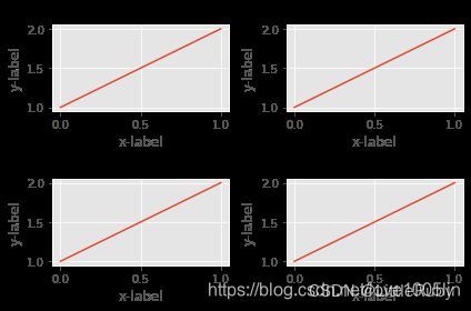
3.3 plt.tight_layout()作用

tight_layout会自动调整子图参数，使之填充整个图像区域。这是个实验特性，可能在一些情况下不工作。它仅仅检查坐标轴标签、刻度标签以及标题的部分。

当你拥有多个子图时，你会经常看到不同轴域的标签叠在一起。

plt.rcParams['savefig.facecolor'] = "0.8"

def example_plot(ax, fontsize=12):
     ax.plot([1, 2])
     ax.locator_params(nbins=3)
     ax.set_xlabel('x-label', fontsize=fontsize)
     ax.set_ylabel('y-label', fontsize=fontsize)
     ax.set_title('Title', fontsize=fontsize)

plt.close('all')
fig, ((ax1, ax2), (ax3, ax4)) = plt.subplots(nrows=2, ncols=2)
example_plot(ax1)
example_plot(ax2)
example_plot(ax3)
example_plot(ax4)

产生图片：

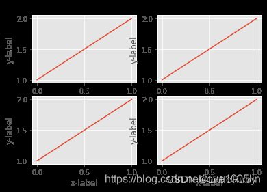
增加plt.tight_layout()会调整子图之间的间隔来减少堆叠。

参考链接：plt.tight_layout()

3.4 x.view()函数

在构建神经网络的时候，经常会用到x.view()函数，实际上view（）类似于reshape（）的用法，将张量重新规划格式，本文将简单介绍这个函数的用法。

import torch

a = torch.arange(1,17)
print(a.shape)
print(a)
a = a.view(-1,4)
print(a.shape)
print(a)

输出

torch.Size([16])
tensor([ 1,  2,  3,  4,  5,  6,  7,  8,  9, 10, 11, 12, 13, 14, 15, 16])
torch.Size([4, 4])
tensor([[ 1,  2,  3,  4],
        [ 5,  6,  7,  8],
        [ 9, 10, 11, 12],
        [13, 14, 15, 16]])

这里view的第一个参数有时会是-1，-1代表不确定，行数将由张量的长度除以列数决定，也就是说
a.view(-1,4) == a.view(4,4)
a.view(-1,8) == a.view(2,8)

参考链接：x.view(-1,4)

3.5 The freeze_support error解决方案

RuntimeError:
       An attempt has been made to start a new process before the
       current process has finished its bootstrapping phase.

   This probably means that you are not using fork to start your
   child processes and you have forgotten to use the proper idiom
   in the main module:

       if __name__ == '__main__':
           freeze_support()
           ...

   The "freeze_support()" line can be omitted if the program
   is not going to be frozen to produce an executable.

这个错误相信很多人都碰到过，就是，在Linux中可以很好运行的代码，在Windows中会给出这样的错误。
究其原因，往往出现在multiprocess上。当程序中调用 multiprocess函数，却不是在main中时，会出现这样的报错。

解决方案：
写一个main函数，然后在if name == ‘main’:中运行这个main函数。把那些引用multiprocessing的函数作都放到main()函数里去执行就OK了。
参考链接：Windows freeze_support Error: An attempt has been made to start a new process

3.6 提升测试acc–改变优化器

原文优化器设置为SDG

opt = torch.optim.Adam(model.parameters(), lr=learn_rate) 

变更优化器为Adam后，代码如下

opt = torch.optim.Adam(model.parameters(), lr=learn_rate) 

变更后，测试精度提升

Epoch: 2, Train_acc:84.2%, Train_loss:0.435, Test_acc:90.2%，Test_loss:0.257
Epoch: 3, Train_acc:89.1%, Train_loss:0.323, Test_acc:84.9%，Test_loss:0.481
Epoch: 4, Train_acc:89.3%, Train_loss:0.346, Test_acc:91.6%，Test_loss:0.218
Epoch: 5, Train_acc:91.3%, Train_loss:0.272, Test_acc:92.9%，Test_loss:0.271
Epoch: 6, Train_acc:96.9%, Train_loss:0.183, Test_acc:94.7%，Test_loss:0.184
Epoch: 7, Train_acc:93.8%, Train_loss:0.261, Test_acc:92.0%，Test_loss:0.312
Epoch: 8, Train_acc:95.6%, Train_loss:0.141, Test_acc:92.4%，Test_loss:0.203
Epoch: 9, Train_acc:97.2%, Train_loss:0.143, Test_acc:94.2%，Test_loss:0.170
Epoch:10, Train_acc:93.1%, Train_loss:0.224, Test_acc:93.8%，Test_loss:0.265
Epoch:11, Train_acc:95.3%, Train_loss:0.275, Test_acc:93.8%，Test_loss:0.211
Epoch:12, Train_acc:95.6%, Train_loss:0.164, Test_acc:94.7%，Test_loss:0.196
Epoch:13, Train_acc:98.2%, Train_loss:0.066, Test_acc:93.3%，Test_loss:0.432
Epoch:14, Train_acc:99.0%, Train_loss:0.052, Test_acc:95.1%，Test_loss:0.191
Epoch:15, Train_acc:98.7%, Train_loss:0.087, Test_acc:93.3%，Test_loss:0.248
Epoch:16, Train_acc:96.8%, Train_loss:0.156, Test_acc:93.8%，Test_loss:0.290
Epoch:17, Train_acc:97.7%, Train_loss:0.067, Test_acc:93.8%，Test_loss:0.268
Epoch:18, Train_acc:99.1%, Train_loss:0.036, Test_acc:94.7%，Test_loss:0.388
Epoch:19, Train_acc:99.6%, Train_loss:0.021, Test_acc:95.6%，Test_loss:0.176
Epoch:20, Train_acc:99.9%, Train_loss:0.012, Test_acc:95.1%，Test_loss:0.181
Done

优化器的详解可以参考链接深度学习 Day11——T11优化器对比实验

总结

通过本文的学习，遇到The freeze_support error问题，网上检索该问题解决方案，顺利解决该问题，并通过改变优化器的方式，提升了原有模型的测试精度。