The Annotated Transformer的中文教程

The Annotated Transformer

Attention is All You Need

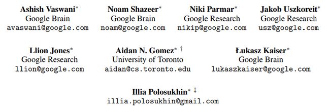
• v2022: Austin Huang, Suraj Subramanian, Jonathan Sum, Khalid Almubarak,
  and Stella Biderman.
• Original:
  Sasha Rush.

The Transformer has been on a lot of
people’s minds over the last five years.
This post presents an annotated version of the paper in the form of a line-by-line implementation. It reorders and deletes some sections from the original paper and adds comments throughout. This document itself is a working notebook, and should be a completely usable implementation. Code is available here.
在过去的五年里，Transformer 一直是很多人关注的焦点。这篇文章以逐行实现的形式呈现了论文的带注释版本。它重新排序并删除了原始论文中的一些部分，并在全文中添加了评论。本文档本身是一个notebook ，并且应该是一个完全可用的实现。代码可以在这里找到。

Table of Contents

• Prelims
• Background
• Part 1: Model Architecture
• Model Architecture
  • Encoder and Decoder Stacks
  • Position-wise Feed-Forward Networks
  • Embeddings and Softmax
  • Positional Encoding
  • Full Model
  • Inference:
• Part 2: Model Training
• Training
  • Batches and Masking
  • Training Loop
  • Training Data and Batching
  • Hardware and Schedule
  • Optimizer
  • Regularization
• A First Example
  • Synthetic Data
  • Loss Computation
  • Greedy Decoding
• Part 3: A Real World Example
  • Data Loading
  • Iterators
  • Training the System
• Additional Components: BPE, Search, Averaging
• Results
  • Attention Visualization
  • Encoder Self Attention
  • Decoder Self Attention
  • Decoder Src Attention
• Conclusion

Prelims 预备

Skip

# !pip install -r requirements.txt

# # Uncomment for colab
# #
# !pip install -q torchdata==0.3.0 torchtext==0.12 spacy==3.2 altair GPUtil
# !python -m spacy download de_core_news_sm
# !python -m spacy download en_core_web_sm

import os
from os.path import exists
import torch
import torch.nn as nn
from torch.nn.functional import log_softmax, pad
import math
import copy
import time
from torch.optim.lr_scheduler import LambdaLR
import pandas as pd
import altair as alt
from torchtext.data.functional import to_map_style_dataset
from torch.utils.data import DataLoader
from torchtext.vocab import build_vocab_from_iterator
import torchtext.datasets as datasets
import spacy
import GPUtil
import warnings
from torch.utils.data.distributed import DistributedSampler
import torch.distributed as dist
import torch.multiprocessing as mp
from torch.nn.parallel import DistributedDataParallel as DDP


# Set to False to skip notebook execution (e.g. for debugging)
# 设置为 False 以跳过notebook 执行（例如用于调试）
warnings.filterwarnings("ignore")
RUN_EXAMPLES = True

# Some convenience helper functions used throughout the notebook
# 整个notebook中使用的一些方便的辅助功能


def is_interactive_notebook():
    return __name__ == "__main__"


def show_example(fn, args=[]):
    if __name__ == "__main__" and RUN_EXAMPLES:
        return fn(*args)


def execute_example(fn, args=[]):
    if __name__ == "__main__" and RUN_EXAMPLES:
        fn(*args)


class DummyOptimizer(torch.optim.Optimizer):
    def __init__(self):
        self.param_groups = [{"lr": 0}]
        None

    def step(self):
        None

    def zero_grad(self, set_to_none=False):
        None


class DummyScheduler:
    def step(self):
        None

My comments are blockquoted. The main text is all from the paper itself.
我的评论被块引用了。正文全部来自论文本身。

Background

减少顺序计算的目标也构成了扩展神经 GPU、ByteNet 和 ConvS2S 的基础，所有这些都使用卷积神经网络作为基本构建块，并行计算所有输入和输出位置的隐藏表示。在这些模型中，关联来自两个任意输入或输出位置的信号所需的操作数量随着位置之间的距离而增加，对于 ConvS2S 呈线性增长，对于 ByteNet 呈对数增长。这使得学习远距离位置之间的依赖关系变得更加困难。在 Transformer 中，这被减少到恒定数量的操作，尽管由于平均注意力加权位置而导致有效分辨率降低，我们用多头注意力来抵消这种影响。

自注意力（有时称为内部注意力）是一种将单个序列的不同位置相关联的注意力机制，以便计算序列的表示。自注意力已成功应用于各种任务，包括阅读理解、抽象概括、文本蕴涵和学习任务无关的句子表示。端到端记忆网络基于循环注意机制而不是序列对齐循环，并且已被证明在简单语言问答和语言建模任务上表现良好。

然而，据我们所知，Transformer 是第一个完全依赖自注意力来计算其输入和输出表示而不使用序列对齐 RNN 或卷积的转换模型。

Part 1: Model Architecture

Model Architecture

Most competitive neural sequence transduction models have an encoder-decoder structure(cite). Here, the encoder maps an input sequence of symbol representations $(x_1,...,x_n)$ to a sequence of continuous representations $\mathbf{z}=(z_1,...,z_n)$. Given $\mathbf{z}$, the decoder then generates an output sequence $(y_1,...,y_m)$ of symbols one element at a time. At each step the model is auto-regressive (cite), consuming the previously generated symbols as additional input when generating the next.

大多数竞争性神经序列转导模型都具有编码器-解码器结构(cite)。这里，编码器将符号表示的输入序列 $(x_1,...,x_n)$ 映射到连续表示序列 $\mathbf{z}=(z_1,...,z_n)$。给定 $\mathbf{z}$，解码器然后生成一个符号输出序列 $(y_1,...,y_m)$，一次一个元素。在每个步骤中，模型都是自回归的(cite)，在生成下一个符号时将先前生成的符号用作附加输入。

class EncoderDecoder(nn.Module):
    """
    A standard Encoder-Decoder architecture. Base for this and many other models.
    标准编码器-解码器架构。该模型和许多其他模型的基础。
    """

    def __init__(self, encoder, decoder, src_embed, tgt_embed, generator):
        super(EncoderDecoder, self).__init__()
        self.encoder = encoder
        self.decoder = decoder
        self.src_embed = src_embed
        self.tgt_embed = tgt_embed
        self.generator = generator

    def forward(self, src, tgt, src_mask, tgt_mask):
        "Take in and process masked src and target sequences."
        "接收并处理屏蔽的源序列和目标序列。"
        return self.decode(self.encode(src, src_mask), src_mask, tgt, tgt_mask)

    def encode(self, src, src_mask):
        return self.encoder(self.src_embed(src), src_mask)

    def decode(self, memory, src_mask, tgt, tgt_mask):
        return self.decoder(self.tgt_embed(tgt), memory, src_mask, tgt_mask)

class Generator(nn.Module):
    "Define standard linear + softmax generation step."
	"定义标准线性+softmax生成步骤。"
    def __init__(self, d_model, vocab):
        super(Generator, self).__init__()
        self.proj = nn.Linear(d_model, vocab)

    def forward(self, x):
        return log_softmax(self.proj(x), dim=-1)

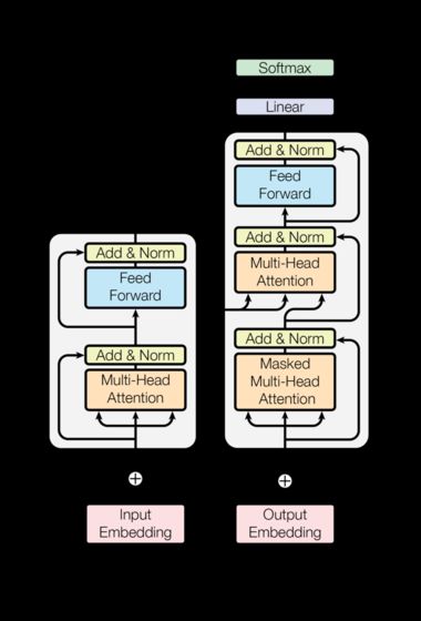
The Transformer follows this overall architecture using stacked self-attention and point-wise, fully connected layers for both the encoder and decoder, shown in the left and right halves of Figure 1, respectively.
Transformer 遵循这一整体架构，对编码器和解码器使用堆叠自注意力和逐点、全连接层，分别如图1的左半部分和右半部分所示。

Encoder and Decoder Stacks编码器和解码器堆栈

Encoder编码器

The encoder is composed of a stack of $N=6$ identical layers.
编码器由 $N=6$ 个相同层的堆栈组成。

def clones(module, N):
    "Produce N identical layers."
    "产生 N 个相同的层。"
    return nn.ModuleList([copy.deepcopy(module) for _ in range(N)])

class Encoder(nn.Module):
    "Core encoder is a stack of N layers"
    "核心编码器是 N 层的堆栈"

    def __init__(self, layer, N):
        super(Encoder, self).__init__()
        self.layers = clones(layer, N)
        self.norm = LayerNorm(layer.size)

    def forward(self, x, mask):
        "Pass the input (and mask) through each layer in turn."
        "将输入（和掩码）依次通过每一层。"
        for layer in self.layers:
            x = layer(x, mask)
        return self.norm(x)

We employ a residual connection(cite) around each of the two sub-layers, followed by layer normalization(cite).
我们在两个子层周围采用残差连接(cite)，然后进行层归一化(cite)。

class LayerNorm(nn.Module):
    "Construct a layernorm module (See citation for details)."
    "构建一个 Layernorm 模块（详细信息请参阅引文）。"
    def __init__(self, features, eps=1e-6):
        super(LayerNorm, self).__init__()
        self.a_2 = nn.Parameter(torch.ones(features))
        self.b_2 = nn.Parameter(torch.zeros(features))
        self.eps = eps

    def forward(self, x):
        mean = x.mean(-1, keepdim=True)
        std = x.std(-1, keepdim=True)
        return self.a_2 * (x - mean) / (std + self.eps) + self.b_2

That is, the output of each sub-layer is $\mathrm{LayerNorm}(x+\mathrm{Sublayer}(x))$, where $\mathrm{Sublayer}(x)$ is the function implemented by the sub-layer itself. We apply dropout (cite) to the output of each sub-layer, before it is added to the sub-layer input and normalized.
也就是说，每个子层的输出为$\mathrm{LayerNorm}(x+\mathrm{Sublayer}(x))$，其中$\mathrm{Sublayer}(x)$是子层实现的函数层本身。我们将 dropout (cite) 应用于每个子层的输出，然后将其添加到子层输入并进行归一化。

To facilitate these residual connections, all sub-layers in the model, as well as the embedding layers, produce outputs of dimension $d_{\text{model}}=512$.
为了促进这些残差连接，模型中的所有子层以及嵌入层都会产生维度 $d_{\text{model}}=512$ 的输出。

class SublayerConnection(nn.Module):
    """
    A residual connection followed by a layer norm.Note for code simplicity the norm is first as opposed to last.
    后面跟着层规范的残差连接。请注意，为了简化代码，norm是第一个，而不是最后一个。
    """

    def __init__(self, size, dropout):
        super(SublayerConnection, self).__init__()
        self.norm = LayerNorm(size)
        self.dropout = nn.Dropout(dropout)

    def forward(self, x, sublayer):
        "Apply residual connection to any sublayer with the same size."
        "将残余连接应用于具有相同尺寸的任何子层。"
        return x + self.dropout(sublayer(self.norm(x)))

Each layer has two sub-layers. The first is a multi-head self-attention mechanism, and the second is a simple, position-wise fully connected feed-forward network.
每层有两个子层。第一种是多头自注意机制，第二种是简单的位置全连接前馈网络。

class EncoderLayer(nn.Module):
    "Encoder is made up of self-attn and feed forward (defined below)"
    "编码器由自attn和前馈（定义如下）组成"

    def __init__(self, size, self_attn, feed_forward, dropout):
        super(EncoderLayer, self).__init__()
        self.self_attn = self_attn
        self.feed_forward = feed_forward
        self.sublayer = clones(SublayerConnection(size, dropout), 2)
        self.size = size

    def forward(self, x, mask):
        "Follow Figure 1 (left) for connections."
        "按照图1（左）进行连接。"
        x = self.sublayer[0](x, lambda x: self.self_attn(x, x, x, mask))
        return self.sublayer[1](x, self.feed_forward)

Decoder解码器

The decoder is also composed of a stack of $N=6$ identical layers.
解码器也由$N＝6$个相同层的堆栈组成。

class Decoder(nn.Module):
    "Generic N layer decoder with masking."
    "带掩码的通用N层解码器。"
    def __init__(self, layer, N):
        super(Decoder, self).__init__()
        self.layers = clones(layer, N)
        self.norm = LayerNorm(layer.size)

    def forward(self, x, memory, src_mask, tgt_mask):
        for layer in self.layers:
            x = layer(x, memory, src_mask, tgt_mask)
        return self.norm(x)

In addition to the two sub-layers in each encoder layer, the decoder inserts a third sub-layer, which performs multi-head attention over the output of the encoder stack. Similar to the encoder, we employ residual connections around each of the sub-layers, followed by layer normalization.
除了每个编码器层中的两个子层之外，解码器还插入第三个子层，该第三子层对编码器堆栈的输出执行多头关注。与编码器类似，我们在每个子层周围使用残差连接，然后进行层归一化。

class DecoderLayer(nn.Module):
    "Decoder is made of self-attn, src-attn, and feed forward (defined below)"
    "解码器由self-attn、src-attn和前馈（定义如下）组成"
    def __init__(self, size, self_attn, src_attn, feed_forward, dropout):
        super(DecoderLayer, self).__init__()
        self.size = size
        self.self_attn = self_attn
        self.src_attn = src_attn
        self.feed_forward = feed_forward
        self.sublayer = clones(SublayerConnection(size, dropout), 3)

    def forward(self, x, memory, src_mask, tgt_mask):
        "Follow Figure 1 (right) for connections."
        "按照图1（右）进行连接。"
        m = memory
        x = self.sublayer[0](x, lambda x: self.self_attn(x, x, x, tgt_mask))
        x = self.sublayer[1](x, lambda x: self.src_attn(x, m, m, src_mask))
        return self.sublayer[2](x, self.feed_forward)

We also modify the self-attention sub-layer in the decoder stack to prevent positions from attending to subsequent positions. This masking, combined with fact that the output embeddings are offset by one position, ensures that the predictions for position $i$ can depend only on the known outputs at positions less than $i$.
我们还修改了解码器堆栈中的自注意子层，以防止位置关注后续位置。这种掩蔽，再加上输出嵌入偏移一个位置的事实，确保了对位置$i$的预测只能取决于小于$i$位置的已知输出。

def subsequent_mask(size):
    "Mask out subsequent positions."
    "掩盖后续位置。"
    attn_shape = (1, size, size)
    subsequent_mask = torch.triu(torch.ones(attn_shape), diagonal=1).type(
        torch.uint8
    )
    return subsequent_mask == 0

Below the attention mask shows the position each tgt word (row) is allowed to look at (column). Words are blocked for attending to future words during training.
注意掩码下面显示了允许每个tgt单词（行）查看（列）的位置。在训练过程中，单词会被阻止以处理将来的单词。

def example_mask():
    LS_data = pd.concat(
        [
            pd.DataFrame(
                {
                    "Subsequent Mask": subsequent_mask(20)[0][x, y].flatten(),
                    "Window": y,
                    "Masking": x,
                }
            )
            for y in range(20)
            for x in range(20)
        ]
    )

    return (
        alt.Chart(LS_data)
        .mark_rect()
        .properties(height=250, width=250)
        .encode(
            alt.X("Window:O"),
            alt.Y("Masking:O"),
            alt.Color("Subsequent Mask:Q", scale=alt.Scale(scheme="viridis")),
        )
        .interactive()
    )


show_example(example_mask)

Attention注意

An attention function can be described as mapping a query and a set of key-value pairs to an output, where the query, keys, values, and output are all vectors. The output is computed as a weighted sum of the values, where the weight assigned to each value is computed by a compatibility function of the query with the corresponding key.

We call our particular attention “Scaled Dot-Product Attention”. The input consists of queries and keys of dimension $d_k$, and values of dimension $d_v$. We compute the dot products of the query
with all keys, divide each by $\sqrt{d_k}$, and apply a softmax function to obtain the weights on the values.

注意力函数可以描述为将查询和一组键值对映射到输出，其中查询、键、值和输出都是向量。输出被计算为值的加权和，其中分配给每个值的权重由查询与相应关键字的兼容性函数计算。
我们将我们的特别关注称为“标度点产品关注”。输入由维度$d_k$的查询和键以及维度$d_v$的值组成。我们计算查询的点积
对于所有键，将每个键除以$\sqrt{｛}{d}_k｝$，并应用softmax函数来获得值的权重。

In practice, we compute the attention function on a set of queries simultaneously, packed together into a matrix $Q$. The keys and values are also packed together into matrices $K$ and $V$. We compute the matrix of outputs as:
在实践中，我们同时计算一组查询的注意力函数，这些查询被打包成矩阵$Q$。键和值也被打包到矩阵$K$和$V$中。我们将输出矩阵计算为：
$$\mathrm{Attention}(Q,K,V)=\mathrm{softmax}(\frac{Q{K}^T}{\sqrt{d_k}})V$$

def attention(query, key, value, mask=None, dropout=None):
    "Compute 'Scaled Dot Product Attention'"
    "计算“标度点积注意力”"
    d_k = query.size(-1)
    scores = torch.matmul(query, key.transpose(-2, -1)) / math.sqrt(d_k)
    if mask is not None:
        scores = scores.masked_fill(mask == 0, -1e9)
    p_attn = scores.softmax(dim=-1)
    if dropout is not None:
        p_attn = dropout(p_attn)
    return torch.matmul(p_attn, value), p_attn

The two most commonly used attention functions are additive attention (cite), and dot-product (multiplicative) attention. Dot-product attention is identical to our algorithm, except for the scaling factor of $\frac{1}{\sqrt{d_k}}$. Additive attention computes the compatibility function using a feed-forward network with a single hidden layer. While the two are similar in theoretical complexity,dot-product attention is much faster and more space-efficient in practice, since it can be implemented using highly optimized matrix multiplication code.
两个最常用的注意力函数是加性注意力(cite)和点积（乘法）注意力。除了$\frac{1}{\sqrt{d_k}}$的比例因子外，点积注意力与我们的算法完全相同。加性注意力使用具有单个隐藏层的前馈网络来计算兼容性函数。虽然两者在理论复杂性上相似，但点积注意力在实践中要快得多，空间效率更高，因为它可以使用高度优化的矩阵乘法代码来实现。

While for small values of $d_k$ the two mechanisms perform similarly, additive attention outperforms dot product attention without scaling for larger values of $d_k$ (cite). We suspect that for large values of $d_k$, the dot products grow large in magnitude, pushing the softmax function into regions where it has extremely small gradients (To illustrate why the dot products get large, assume that the components of $q$ and $k$ are independent random variables with mean $0$ and variance $1$. Then their dot product, $q\cdot k={\sum }_{i=1}^{d_k}{q}_i{k}_i$, has mean $0$ and variance $d_k$.). To counteract this effect, we scale the dot products by $\frac{1}{\sqrt{d_k}}$.
虽然对于较小的$d_k$值，这两种机制表现相似，但在不缩放较大的$d_k$(cite)值的情况下，加性注意力优于点积注意力，将softmax函数推送到梯度极小的区域（为了说明点积变大的原因，假设$q$和$k$的分量是独立的随机变量，平均值为$0$，方差为$1$。那么它们的点积$q\cdot k={\sum }_{i=1}^{d_k}{q}_i{k}_i$的平均值为$0$，方差值为$d_k$。）。为了抵消这种影响，我们按$\frac{1}{\sqrt{d_k}}$缩放点积。

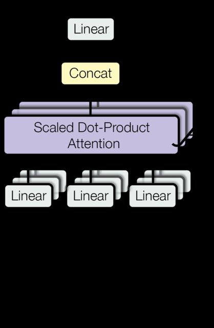
Multi-head attention allows the model to jointly attend to information from different representation subspaces at different positions. With a single attention head, averaging inhibits this.
多头注意力允许模型联合关注来自不同位置的不同表示子空间的信息。对于一个注意力集中的头部，平均值会抑制这种情况。

$$\begin{gathered} \mathrm{MultiHead}(Q,K,V)=\mathrm{Concat}(\mathrm{hea}{\mathrm{d}}_1,...,\mathrm{hea}{\mathrm{d}}_{\mathrm{h}})W^O \\ \text{where}\mathrm{hea}{\mathrm{d}}_{\mathrm{i}}=\mathrm{Attention}(Q{W}_i^Q,K{W}_i^K,V{W}_i^V) \end{gathered}$$

Where the projections are parameter matrices（其中投影是参数矩阵 ）
$W_i^Q\in {\mathbb{R}}^{d_{\text{model}}\times d_k}$, $W_i^K\in {\mathbb{R}}^{d_{\text{model}}\times d_k}$, $W_i^V\in {\mathbb{R}}^{d_{\text{model}}\times d_v}$ and $W^O\in {\mathbb{R}}^{h{d}_v\times d_{\text{model}}}$.

In this work we employ $h=8$ parallel attention layers, or heads. For each of these we use $d_k=d_v=d_{\text{model}}/h=64$. Due to the reduced dimension of each head, the total computational cost is similar to that of single-head attention with full dimensionality.
在这项工作中，我们采用 $h=8$ 并行注意力层或头。对于每一个，我们使用 $d_k=d_v=d_{\text{model}}/h=64$。由于每个头的维度减少，总计算成本与全维度的单头注意力相似。

class MultiHeadedAttention(nn.Module):
    def __init__(self, h, d_model, dropout=0.1):
        "Take in model size and number of heads."
        "考虑模型尺寸和头数。"
        super(MultiHeadedAttention, self).__init__()
        assert d_model % h == 0
        # We assume d_v always equals d_k 
        # 我们假设 d_v 始终等于 d_k
        self.d_k = d_model // h
        self.h = h
        self.linears = clones(nn.Linear(d_model, d_model), 4)
        self.attn = None
        self.dropout = nn.Dropout(p=dropout)

    def forward(self, query, key, value, mask=None):
        "Implements Figure 2 "
        "实现图 2"
        if mask is not None:
            # Same mask applied to all h heads.
            mask = mask.unsqueeze(1)
        nbatches = query.size(0)

        # 1) Do all the linear projections in batch from d_model => h x d_k
        # 1）从 d_model => h x d_k 批量进行所有线性投影
        query, key, value = [
            lin(x).view(nbatches, -1, self.h, self.d_k).transpose(1, 2)
            for lin, x in zip(self.linears, (query, key, value))
        ]

        # 2) Apply attention on all the projected vectors in batch.
        # 2）批量关注所有投影向量。
        x, self.attn = attention(
            query, key, value, mask=mask, dropout=self.dropout
        )

        # 3) "Concat" using a view and apply a final linear.
        # 3) 使用视图“连接”并应用最终的线性。
        x = (
            x.transpose(1, 2)
            .contiguous()
            .view(nbatches, -1, self.h * self.d_k)
        )
        del query
        del key
        del value
        return self.linears[-1](x)

Applications of Attention in our Model 注意力在我们模型中的应用

The Transformer uses multi-head attention in three different ways:
Transformer 以三种不同的方式使用多头注意力：

1. In “encoder-decoder attention” layers, the queries come from the previous decoder layer, and the memory keys and values come from the output of the encoder. This allows every position in the decoder to attend over all positions in the input sequence. This mimics the typical encoder-decoder attention mechanisms in sequence-to-sequence models such as (cite).1) 在“编码器-解码器注意”层中，查询来自前一个解码器层，内存键和值来自编码器的输出。这允许解码器中的每个位置都参与输入序列中的所有位置。这模仿了序列到序列模型中典型的编码器-解码器注意机制，例如(cite)。

2. The encoder contains self-attention layers. In a self-attention layer all of the keys, values and queries come from the same place, in this case, the output of the previous layer in the encoder. Each position in the encoder can attend to all positions in the previous layer of the encoder.2) 编码器包含自注意力层。在自注意力层中，所有键、值和查询都来自同一位置，在本例中是编码器中前一层的输出。编码器中的每个位置可以关注编码器上一层中的所有位置。

3. Similarly, self-attention layers in the decoder allow each position in the decoder to attend to all positions in the decoder up to and including that position. We need to prevent leftward information flow in the decoder to preserve the auto-regressive property. We implement this inside of scaled dot-product attention by masking out (setting to $-\infty$) all values in the input of the softmax which correspond to illegal connections. 3) 类似地，解码器中的自注意力层允许解码器中的每个位置关注解码器中直到并包括该位置的所有位置。我们需要防止解码器中的左向信息流以保留自回归属性。我们通过屏蔽（设置为 $-\infty$）softmax 输入中与非法连接相对应的所有值，在缩放点积注意力内部实现这一点。