Support Vector Machine 建模（基于三种数据集）

目录

一、 SVM 对于 Iris 数据集的处理

建模： 

二、 SVM 对于 弯月数据集的处理

建模：

三、 SVM 对于 direct marketing campaigns (phone calls)数据集的处理

 建模：

Support Vector Machine (SVM)是一种机器学习算法，属于监督学习方法。它在分类和回归问题中广泛应用。

SVM的目标是将数据集划分为不同的类别，并且找到一个最优的超平面，使得不同类别的样本在超平面上的投影点尽可能地分离开来。超平面可以被看作是一个分割数据空间的决策边界。SVM在划分决策边界时，会选取能够最大化边界到最近样本点（称为支持向量）的距离的超平面。

SVM的主要优点是可以处理高维数据和非线性问题，并且对于训练样本数量相对较少的情况下也能有较好的表现。它可以通过使用不同的核函数来应用于非线性分类和回归问题，如线性核、多项式核、高斯核等。

SVM的训练过程可以通过求解一个二次规划问题来实现，该问题的目标是最大化边界的宽度，同时使得分类误差最小化。在求解过程中，只有支持向量（离超平面最近的样本点）对最终分类结果有影响，而其他样本点对最终结果没有影响，这使得SVM具有较好的鲁棒性。

支持向量机的优势在于：

1. 可以解决高维空间中的非线性问题。
2. 在训练过程中只使用了支持向量，大大减少了存储和计算的开销。
3. 在样本数量较少的情况下，也能够得到较好的分类效果。

支持向量机在不同的问题中有多种变体，包括线性支持向量机（Linear SVM）、非线性支持向量机（Nonlinear SVM）、多类别支持向量机等。它在模式识别、文本分类、图像识别等领域具有广泛的应用。

import numpy as np # linear algebra
import pandas as pd # data processing, CSV file I/O (e.g. pd.read_csv)
import matplotlib.pyplot as plt
import seaborn as sns
from sklearn.preprocessing import PolynomialFeatures, StandardScaler
from sklearn.svm import LinearSVC
from sklearn.svm import SVC
from sklearn.model_selection import train_test_split

一、 SVM 对于 Iris 数据集的处理

from sklearn import datasets 
iris = datasets.load_iris()#引用数据

X = iris['data'][:,(2,3)]

scaler = StandardScaler()
Xstan = scaler.fit_transform(X)#数据标准化

data = pd.DataFrame(data=Xstan, columns=['petal length','petal width'])#这两种区分比较明显
data['target'] = iris['target']
data = data[data['target']!=2] # we will only focus on Iris-setosa and Iris-Versicolor
data#去掉了target==2的情况

sns.lmplot(x='petal length',y='petal width',hue='target',data=data, fit_reg=False, legend=False)

plt.legend(['Iris-Setosa','Iris-Versicolor'], fontsize = 14)
plt.xlabel('petal length (scaled)', fontsize = 18)
plt.ylabel('petal width (scaled)', fontsize = 18)
plt.show()

 

svc = LinearSVC(C=1,loss="hinge")
svc.fit(data[['petal length','petal width']].values,data['target'].values)#x,y赋给模型

'''
LinearSVC是一个线性SVM分类器。它有以下几个常用参数：

1. penalty：正则化惩罚的类型。默认为L2正则化。可以选择L1正则化，但通常L2正则化效果更好。

2. loss：损失函数的类型。默认为"l2"损失。可以选择"hinge"损失，即线性SVM的损失函数。

3. dual：计算对偶或原始优化问题。默认为True，即通过对偶问题求解。当样本数大于特征数时，设置为False，使用原始问题求解。

4. C：正则化参数。默认为1.0。C越小，正则化越强，可以减小过拟合的风险。

5. multi_class：多类别分类的策略。默认为"ovr"，即一对多策略。可以选择"crammer_singer"，即多分类的SVC。

6. fit_intercept：是否拟合截距。默认为True。如果数据已经被中心化，则可以设置为False。

7. intercept_scaling：拟合截距的缩放因子。默认为1。

8. class_weight：样本权重。可以给不同类别的样本赋予不同的权重，用于处理不平衡的数据集。

9. random_state：随机种子。默认为None。

这些参数可以根据实际情况进行调整，以获得最佳的模型性能。
'''

# get the parameters
w0,w1 = svc.coef_[0]
b = svc.intercept_[0]

x0 = np.linspace(-1.7, 0.7, num=100)#在-1.7到0.7取100个点
# decision boundary
x1_decision = -b/w1 - w0/w1*x0 #0 = x0*w1 + x1*w1 + b的情况转化而来
# +1 margin
x1_plus = x1_decision + 1/w1#1 = x0*w1 + x1*w1 + b的情况转化而来
# -1 margin 
x1_minus = x1_decision - 1/w1#-1 = x0*w1 + x1*w1 + b的情况转化而来

sns.lmplot(x='petal length',y='petal width',hue='target',data=data, fit_reg=False, legend=False)
plt.plot(x0,x1_decision, color='grey')
plt.plot(x0,x1_plus,x0,x1_minus,color='grey', linestyle='--')
plt.legend(['Iris-Setosa','Iris-Versicolor','decision boundary','margin','margin'], fontsize = 14, loc='center left', bbox_to_anchor=(1.05,0.5))

plt.xlabel('petal length (scaled)', fontsize = 18)
plt.ylabel('petal width (scaled)', fontsize = 18)
plt.title('C = 1', fontsize = 20)
plt.ylim(-1.6,1)
plt.xlim(-1.7,0.8)
plt.show()#c=1可以容忍一些点偏离

建模： 

svc = LinearSVC(C=1000,loss="hinge") # let's change C to a much larger value
svc.fit(data[['petal length','petal width']].values,data['target'].values)

# get the parameters
w0,w1 = svc.coef_[0]
b = svc.intercept_[0]

x0 = np.linspace(-1.7, 0.7, num=100)
# decision boundary
x1_decision = -b/w1 - w0/w1*x0
# +1 margin
x1_plus = x1_decision + 1/w1
# -1 margin 
x1_minus = x1_decision - 1/w1

sns.lmplot(x='petal length',y='petal width',hue='target',data=data, fit_reg=False, legend=False)
plt.plot(x0,x1_decision, color='grey')
plt.plot(x0,x1_plus,x0,x1_minus,color='grey', linestyle='--')
plt.legend(['decision boundary','margin','margin','Iris-Setosa','Iris-Versicolor'], fontsize = 14, loc='center left', bbox_to_anchor=(1.05,0.5))
plt.xlabel('petal length (scaled)', fontsize = 18)
plt.ylabel('petal width (scaled)', fontsize = 18)
plt.title('C = 1000', fontsize = 20)
plt.ylim(-1.6,1)
plt.xlim(-1.7,0.8)
plt.show()#c=1000容忍度小，区分度高

 

二、 SVM 对于 弯月数据集的处理

##SVM 对于 弯月数据集的处理
from sklearn.datasets import make_moons
X,y=make_moons(noise=0.1, random_state=2) #噪音为0.1 # fix random_state to make sure it produces the same dataset everytime. Remove it if you want randomized dataset.
data = pd.DataFrame(data = X, columns=['x1','x2'])
data['y']=y
data.head()

sns.lmplot(x='x1',y='x2',hue='y',data=data, fit_reg=False, legend=True, height=4, aspect=4/3)
plt.xlabel('x1', fontsize = 18)
plt.ylabel('x2', fontsize = 18)
plt.show()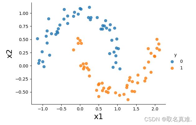

 

# tranform the features, here we use a 3rd degree polynomials
print('Shape of X before tranformation:', X.shape)
poly = PolynomialFeatures(degree = 3, include_bias=False)#多项式为3
Xpoly = poly.fit_transform(X)
print('Shape of X aftere tranformation:', Xpoly.shape)

#结果：Shape of X before tranformation: (100, 2)
#     Shape of X aftere tranformation: (100, 9)

'''
PolynomialFeatures是一个数据预处理工具，用于将原始特征集转换为多项式特征集。它将原始特征的幂次组合成新的特征，以增加模型的非线性能力。

例如，对于一个二维特征集[x1, x2]，使用PolynomialFeatures(degree=2)可以生成如下特征集：[1, x1, x2, x1^2, x1*x2, x2^2]。这样，原始特征集中的每个特征都可以与其他特征相乘或平方，从而产生更多的特征组合。

通过引入多项式特征，PolynomialFeatures可以帮助模型更好地拟合非线性关系。它常常与线性回归、逻辑回归等模型一起使用，以提高模型的性能。
'''

# standardize the data
scaler = StandardScaler()#标准化数据
Xpolystan = scaler.fit_transform(Xpoly)

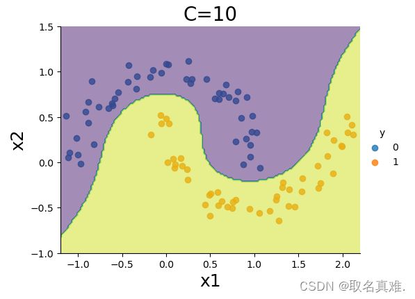
建模：

svm_clf = LinearSVC(C=10,loss='hinge',max_iter=10000)
svm_clf.fit(Xpolystan,y)

def make_meshgrid(x, y, h=.02):
    x_min, x_max = x.min() - 1, x.max() + 1
    y_min, y_max = y.min() - 1, y.max() + 1
    xx, yy = np.meshgrid(np.arange(x_min, x_max, h), np.arange(y_min, y_max, h))
    return xx, yy

# create grids
X0, X1 = X[:, 0], X[:, 1]
xx0, xx1 = make_meshgrid(X0, X1)
# polynomial transformation and standardization on the grids
xgrid = np.c_[xx0.ravel(), xx1.ravel()]
xgridpoly = poly.transform(xgrid)
xgridpolystan = scaler.transform(xgridpoly)
# prediction
Z = xgridpolystan.dot(svm_clf.coef_[0].reshape(-1,1)) + svm_clf.intercept_[0] # wx + b
#Z = svm_clf.predict(xgridpolystan)
Z = Z.reshape(xx0.shape)

# plotting prediction contours - decision boundary (Z=0), and two margins (Z = 1 or -1)
sns.lmplot(x='x1',y='x2',hue='y',data=data, fit_reg=False, legend=True, height=4, aspect=4/3)
CS=plt.contour(xx0, xx1, Z, alpha=0.5, levels=[-1,0,1])
plt.clabel(CS, inline=1,levels=[-1.0,0,1.0], fmt='%1.1f', fontsize=12, manual=[(1.5,0.3),(0.5,0.0),(-0.5,-0.2)])
#
plt.xlim(-1.2,2.2)
plt.ylim(-1,1.5)
plt.title('C=10', fontsize = 20)
plt.xlabel('x1', fontsize = 18)
plt.ylabel('x2', fontsize = 18)
plt.show()

svm_clf = LinearSVC(C=1000,loss='hinge',max_iter=10000)
svm_clf.fit(Xpolystan,y)

# prediction
Z = xgridpolystan.dot(svm_clf.coef_[0].reshape(-1,1)) + svm_clf.intercept_[0] # wx + b
#Z = svm_clf.predict(xgridpolystan)
Z = Z.reshape(xx0.shape)

# plotting prediction contours - decision boundary (Z=0), and two margins (Z = 1 or -1)
sns.lmplot(x='x1',y='x2',hue='y',data=data, fit_reg=False, legend=True, height=4, aspect=4/3)
CS=plt.contour(xx0, xx1, Z, alpha=0.5, levels=[-1,0,1])
plt.clabel(CS, inline=1,levels=[-1.0,0,1.0], fmt='%1.1f', fontsize=12, manual=[(1.5,0.1),(0.5,0.0),(-0.5,0.0)])
plt.xlim(-1.2,2.2)
plt.ylim(-1,1.5)
plt.title('C=1000', fontsize = 20)
plt.xlabel('x1', fontsize = 18)
plt.ylabel('x2', fontsize = 18)
plt.show()

 

from sklearn.svm import SVC

scaler = StandardScaler()
Xstan = scaler.fit_transform(X)
svm_clf = SVC(kernel='poly', degree=3, C=10, coef0=1)
svm_clf.fit(Xstan,y)

# create grids
X0, X1 = X[:, 0], X[:, 1]
xx0, xx1 = make_meshgrid(X0, X1)
# standardization on the grids
xgrid = np.c_[xx0.ravel(), xx1.ravel()]
xgridstan = scaler.transform(xgrid)

# prediction
Z = svm_clf.predict(xgridstan)
Z = Z.reshape(xx0.shape)

# plotting prediction contours - decision boundary (Z=0), and two margins (Z = 1 or -1)
sns.lmplot(x='x1',y='x2',hue='y',data=data, fit_reg=False, legend=True, height=4, aspect=4/3)
plt.contourf(xx0, xx1, Z, alpha=0.5)
plt.xlim(-1.2,2.2)
plt.ylim(-1,1.5)
plt.title('C=10', fontsize = 20)
plt.xlabel('x1', fontsize = 18)
plt.ylabel('x2', fontsize = 18)
plt.show()

 ​​​​​​​

三、 SVM 对于 direct marketing campaigns (phone calls)数据集的处理

data = pd.read_csv('bank-additional-full.csv',sep=';') # note that the delimiter for this dataset is ";"
data = data.drop('duration',axis=1) # as recommended by the dataset description, we will drop the last contact duration values.

header = ['age','campaign','pdays','previous','emp.var.rate','cons.price.idx','cons.conf.idx','euribor3m','nr.employed']
data.hist(column=header,figsize=(10,10))
plt.subplots_adjust(wspace = 0.5, hspace = 0.5)
plt.show()

 

数据转化：

data['poutcome'] = data['poutcome'].map({'failure': -1,'nonexistent': 0,'success': 1})

data['default'] = data['default'].map({'yes': -1,'unknown': 0,'no': 1})
data['housing'] = data['housing'].map({'yes': -1,'unknown': 0,'no': 1})
data['loan'] = data['loan'].map({'yes': -1,'unknown': 0,'no': 1})

nominal = ['job','marital','education','contact','month','day_of_week']
dataProcessed = pd.get_dummies(data,columns=nominal)

dataProcessed['y']=dataProcessed['y'].map({'yes': 1,'no': 0})
dataProcessed.head()#数据转化

# raw data
X = dataProcessed.drop('y', axis=1).values
y = dataProcessed['y'].values
# split, random_state is used for repeatable results, you should remove it if you are running your own code.
X_train, X_test, y_train, y_test = train_test_split(X, y, test_size=0.30, random_state=42)


print('X train size: ', X_train.shape)
print('y train size: ', y_train.shape)
print('X test size: ', X_test.shape)
print('y test size: ', y_test.shape)

# column index of numeric variables 将这几行标准化
idx_numeric=[0,4,5,6,8,9,10,11,12]
##print(dataProcessed.columns[idx])

# standardize numeric variables only
scaler = StandardScaler()
X_train[:,idx_numeric]=scaler.fit_transform(X_train[:,idx_numeric])
X_test[:,idx_numeric]=scaler.transform(X_test[:,idx_numeric])

 建模：

from sklearn.model_selection import GridSearchCV

tuned_parameters = [{'kernel': ['rbf'], 'gamma': [0.1],
                     'C': [1]},
                    {'kernel': ['linear'], 'C': [1]}]

clf = GridSearchCV(SVC(), tuned_parameters, cv=5, scoring='precision')
clf.fit(X_train, y_train)

print(clf.cv_results_)
'''结果：
{'mean_fit_time': array([ 74.57606063, 186.00122666]), 'std_fit_time': array([ 8.75207326, 20.73950882]), 'mean_score_time': array([6.15259757, 1.5593924 ]), 'std_score_time': array([0.20244041, 0.03502866]), 'param_C': masked_array(data=[1, 1],
             mask=[False, False],
       fill_value='?',
            dtype=object), 'param_gamma': masked_array(data=[0.1, --],
             mask=[False,  True],
       fill_value='?',
            dtype=object), 'param_kernel': masked_array(data=['rbf', 'linear'],
             mask=[False, False],
       fill_value='?',
            dtype=object), 'params': [{'C': 1, 'gamma': 0.1, 'kernel': 'rbf'}, {'C': 1, 'kernel': 'linear'}], 'split0_test_score': array([0.66044776, 0.64186047]), 'split1_test_score': array([0.64081633, 0.61320755]), 'split2_test_score': array([0.66396761, 0.64878049]), 'split3_test_score': array([0.68325792, 0.65128205]), 'split4_test_score': array([0.69731801, 0.67924528]), 'mean_test_score': array([0.66916153, 0.64687517]), 'std_test_score': array([0.01948257, 0.02111649]), 'rank_test_score': array([1, 2])}
'''

print('The best model is: ', clf.best_params_)
print('This model produces a mean cross-validated score (precision) of', clf.best_score_)
'''结果：
The best model is:  {'C': 1, 'gamma': 0.1, 'kernel': 'rbf'}
This model produces a mean cross-validated score (precision) of 0.6691615250551093
'''

from sklearn.metrics import precision_score, accuracy_score
y_true, y_pred = y_test, clf.predict(X_test)
print('precision on the evaluation set: ', precision_score(y_true, y_pred))
print('accuracy on the evaluation set: ', accuracy_score(y_true, y_pred))
'''结果：
precision on the evaluation set:  0.647834274952919
accuracy on the evaluation set:  0.9002994254268836
'''